
Universal Relations for Rapidly Rotating Neutron Stars#
Essentials#
import pandas as pd
import numpy as np
from scipy import stats
import os,sys,math
import matplotlib as mpl
from mpl_toolkits.axes_grid1 import Divider, Size
from matplotlib import rc
rc('mathtext', fontset='cm')
import matplotlib.pyplot as plt
import seaborn as sn
from scipy import optimize
from scipy.optimize import curve_fit
from scipy.stats import linregress
from math import log,exp,sqrt,cos,sin
from math import *
from sympy import *
import time
from IPython.display import display, clear_output
from mpl_toolkits.mplot3d import Axes3D
from mpl_toolkits.mplot3d import axes3d
from matplotlib import cm
Scikit learn#
# Pipeline-Linear Regression model
from sklearn.preprocessing import PolynomialFeatures
from sklearn.linear_model import LinearRegression, Lasso
from sklearn.pipeline import Pipeline
#cross validation
from sklearn.model_selection import cross_validate, LeaveOneOut
Constants#
Msun=1.987e33 #gr
Msun_kg=1.987e30 #kg
c=2.9979e10 #cm/sec
G=6.6732e-8 # cm^3/(gr*sec^2)
c_new=2.9979e5 #km/s
G_new=6.6732e-20 #km^3/kg*s^2
Stellar compactness in geometric units: \(C=M/R\)#
Inverse stellar compactness \(\mathcal{K}=C^{-1}\)#
Spin parameter \(\chi=J/M^2\) where \(J\equiv J_{geom} [km^2], \ M\equiv M_{geom} [km]\)#
Reduced spin parameter \(\sigma=\frac{\Omega^{2}R^3}{GM} [-]\)#
Geroch-Hansen quadrupole moment \(M^{GH}_{2} [km^3]\)#
Reduced quadrupole moment \(\bar{Q}=-MM^{GH}_{2}/J^2=-M^{GH}_{2}/\chi^2M^3\)#
Moment of Inertia \(I_{geom}=IG/c^2 \ [km^3],\ \bar{I}=I_{geom}/M_{geom}^3\ [-] \)#
Frequency in geometric units \(\tilde{f}=f(Hz)/c \ [km^{-1}]\)#
\(\frac{1}{2\pi\bar{I}}=\frac{M [km]\times \tilde{f} [km^{-1}]}{\chi}\ [-]\)#
Geroch-Hansen octupole moment: \(S_3 \ [km^4]\)#
Reduced octupole moment: \(\bar{S_3}=-S_{3}/\chi^3M^4\)#
————————————————————–#
Data for rapidly rotating Neutron Stars extracted from RNS source code#
————————————————————–#
# ------------------Hadronic Stars---------------------------
rotation_ski2 = pd.read_csv("./rapidly_ rot _Ns_data/rotation_ski2.txt", sep="\t")
rotation_ski3 = pd.read_csv("./rapidly_ rot _Ns_data/rotation_ski3.txt", sep="\t")
rotation_ski4 = pd.read_csv("./rapidly_ rot _Ns_data/rotation_ski4.txt", sep="\t")
rotation_ski5 = pd.read_csv("./rapidly_ rot _Ns_data/rotation_ski5.txt", sep="\t")
rotation_ski6 = pd.read_csv("./rapidly_ rot _Ns_data/rotation_ski6.txt", sep="\t")
rotation_skop = pd.read_csv("./rapidly_ rot _Ns_data/rotation_skop.txt", sep="\t")
rotation_sly230a = pd.read_csv("./rapidly_ rot _Ns_data/rotation_sly230a.txt", sep="\t")
rotation_kdeov = pd.read_csv("./rapidly_ rot _Ns_data/rotation_kdeov.txt", sep="\t")
rotation_kdeov1 = pd.read_csv("./rapidly_ rot _Ns_data/rotation_kdeov1.txt", sep="\t")
rotation_rs = pd.read_csv("./rapidly_ rot _Ns_data/rotation_rs.txt", sep="\t")
rotation_sk255 = pd.read_csv("./rapidly_ rot _Ns_data/rotation_sk255.txt", sep="\t")
rotation_sk272 = pd.read_csv("./rapidly_ rot _Ns_data/rotation_sk272.txt", sep="\t")
rotation_sly2 = pd.read_csv("./rapidly_ rot _Ns_data/rotation_sly2.txt", sep="\t")
rotation_sly4 = pd.read_csv("./rapidly_ rot _Ns_data/rotation_sly4.txt", sep="\t")
rotation_sly9 = pd.read_csv("./rapidly_ rot _Ns_data/rotation_sly9.txt", sep="\t")
rotation_ska = pd.read_csv("./rapidly_ rot _Ns_data/rotation_ska.txt", sep="\t")
rotation_skb = pd.read_csv("./rapidly_ rot _Ns_data/rotation_skb.txt", sep="\t")
rotation_skmp = pd.read_csv("./rapidly_ rot _Ns_data/rotation_skmp.txt", sep="\t")
rotation_bl_2018 = pd.read_csv("./rapidly_ rot _Ns_data/rotation_bl_2018.txt", sep="\t")
rotation_ddhd = pd.read_csv("./rapidly_ rot _Ns_data/rotation_ddhd.txt", sep="\t")
rotation_ds2 = pd.read_csv("./rapidly_ rot _Ns_data/rotation_ds2.txt", sep="\t")
rotation_ds4 = pd.read_csv("./rapidly_ rot _Ns_data/rotation_ds4.txt", sep="\t")
rotation_ds6 = pd.read_csv("./rapidly_ rot _Ns_data/rotation_ds6.txt", sep="\t")
rotation_ds8 = pd.read_csv("./rapidly_ rot _Ns_data/rotation_ds8.txt", sep="\t")
#-----------------Hyperonic Stars ----------------------------
rotation_dns = pd.read_csv("./rapidly_ rot _Ns_data/rotation_dns.txt", sep="\t")
rotation_ddhdy4 = pd.read_csv("./rapidly_ rot _Ns_data/rotation_ddhdy4.txt", sep="\t")
rotation_ds1 = pd.read_csv("./rapidly_ rot _Ns_data/rotation_ds1.txt", sep="\t")
rotation_ds3 = pd.read_csv("./rapidly_ rot _Ns_data/rotation_ds3.txt", sep="\t")
rotation_ds5 = pd.read_csv("./rapidly_ rot _Ns_data/rotation_ds5.txt", sep="\t")
rotation_ds7 = pd.read_csv("./rapidly_ rot _Ns_data/rotation_ds7.txt", sep="\t")
rotation_gm1y5 = pd.read_csv("./rapidly_ rot _Ns_data/rotation_gm1y5.txt", sep="\t")
rotation_gm1y6 = pd.read_csv("./rapidly_ rot _Ns_data/rotation_gm1y6.txt", sep="\t")
#------------------Hybrid Stars------------------------------
rotation_dd2_2 = pd.read_csv("./rapidly_ rot _Ns_data/rotation_dd2_2.txt", sep="\t")
rotation_dd2_2v = pd.read_csv("./rapidly_ rot _Ns_data/rotation_dd2_2v.txt", sep="\t")
rotation_qhc18 = pd.read_csv("./rapidly_ rot _Ns_data/rotation_qhc18.txt", sep="\t")
rotation_qhc19b = pd.read_csv("./rapidly_ rot _Ns_data/rotation_qhc19b.txt", sep="\t")
rotation_qhc19c = pd.read_csv("./rapidly_ rot _Ns_data/rotation_qhc19c.txt", sep="\t")
rotation_qhc19d = pd.read_csv("./rapidly_ rot _Ns_data/rotation_qhc19d.txt", sep="\t")
———————————————————-#
Functions in python defined#
———————————————————-#
Cross validation pipeline for polynomial model features#
def cross_validation_function(data_frame, x,y,z, pol_degree):
    # Formula to predict and testing the unkown data with leaveout function

    #Data, targets
    train_data = data_frame[[x, y]].to_numpy()
    target = data_frame[z].to_numpy()

    #------Pipeline------------------------
    model = Pipeline([("poly", PolynomialFeatures(degree=pol_degree)),("linear_reg", LinearRegression())])

    # Scores: statistical evaluation score functions from scikit learn
    scores = ["max_error","neg_mean_absolute_error","neg_mean_squared_error","neg_root_mean_squared_error",
              "explained_variance","neg_mean_absolute_percentage_error"]
    cv_results = cross_validate(model, train_data, target, cv=LeaveOneOut(), scoring=scores)

    #------Results at cross-validation saved in Data Fame-----------
    cv_results = pd.DataFrame(cv_results)

    #----Statistical evaluation metric functions----------------
    #---------------calculation---------------------------------
    mean_MAE = (-cv_results['test_neg_mean_absolute_error']).mean()
    mean_MSE = (-cv_results['test_neg_mean_squared_error']).mean()
    max_validation_error = (-cv_results['test_max_error']).max()
    max_relative_valitation_error = (-100*cv_results['test_neg_mean_absolute_percentage_error']).max()
    MAPE_validation_error = (-100*cv_results['test_neg_mean_absolute_percentage_error']).mean()
    explained_variance = (cv_results['test_explained_variance']).mean()
    useful_output_data = np.array([mean_MAE,max_validation_error,mean_MSE,max_relative_valitation_error,
                          MAPE_validation_error,explained_variance,pol_degree])

    #--------------data saved to data frame---------------------------
    useful_data_frame = pd.DataFrame(useful_output_data)
    names = ['MAE','Max_Error','MSE','d(%)','MAPE(%)','Explained_Variance','k']

    #--------------Final output----------------------------------------
    validation_evaluation_metrics = pd.DataFrame(useful_data_frame.values.reshape(1,7), columns = names)


    return cv_results, validation_evaluation_metrics, useful_output_data
def cross_validation_function_2(data_frame, x,z, pol_degree):
    # Formula to predict and testing the unkown data with leaveout function

    #Data, targets
    train_data = data_frame[[x]].to_numpy()
    target = data_frame[z].to_numpy()

    #------Pipeline------------------------
    model = Pipeline([("poly", PolynomialFeatures(degree=pol_degree)),("linear_reg", LinearRegression())])

    # Scores: statistical evaluation score functions from scikit learn
    scores = ["max_error","neg_mean_absolute_error","neg_mean_squared_error","neg_root_mean_squared_error",
              "explained_variance","neg_mean_absolute_percentage_error"]
    cv_results = cross_validate(model, train_data, target, cv=LeaveOneOut(), scoring=scores)

    #-------Results at cross-validation saved in Data Fame------
    cv_results = pd.DataFrame(cv_results)

    #----Statistical evaluation metric functions----------------
    #----------------calcuation---------------------------------
    mean_MAE = (-cv_results['test_neg_mean_absolute_error']).mean()
    mean_MSE = (-cv_results['test_neg_mean_squared_error']).mean()
    max_validation_error = (-cv_results['test_max_error']).max()
    max_relative_valitation_error = (-100*cv_results['test_neg_mean_absolute_percentage_error']).max()
    MAPE_validation_error = (-100*cv_results['test_neg_mean_absolute_percentage_error']).mean()
    explained_variance = (cv_results['test_explained_variance']).mean()
    useful_output_data = np.array([mean_MAE,max_validation_error,mean_MSE,max_relative_valitation_error,
                          MAPE_validation_error,explained_variance,pol_degree])

    #--------------data saved to dataframe-----------------------
    useful_data_frame = pd.DataFrame(useful_output_data)
    names = ['MAE','Max_Error','MSE','d(%)','MAPE(%)','Explained_Variance','k']

    #--------------Final output----------------------------------
    validation_evaluation_metrics = pd.DataFrame(useful_data_frame.values.reshape(1,7), columns = names)


    return cv_results, validation_evaluation_metrics,useful_output_data
def c_val_performace_results_for_k(df,x,y,z):
    stat_metric_list_at_cv = list()
    for i in range(2,8):
        #print(f'Order of the polynomial function: {i}')
        performance_results_at_cv = cross_validation_function(df, x = x,y= y ,z=z, pol_degree=i)
        #print(performance_results_at_cv[1])
        stat_metric_list_at_cv.append(performance_results_at_cv[2])

    names = ['MAE','Max_Error','MSE','d(%)','MAPE(%)','Explained_Variance','k']
    df = pd.DataFrame(stat_metric_list_at_cv, columns =names)
    return df
#df_new.to_csv(r'kde0v.txt',header=None,index=None,float_format='%.15e',sep=' ')
def c_val_performace_results_for_k_2(df,x,z):
    stat_metric_list_at_cv = list()
    for i in range(2,8):
        #print(f'Order of the polynomial function: {i}')
        performance_results_at_cv = cross_validation_function_2(df, x = x ,z=z, pol_degree=i)
        #print(performance_results_at_cv[1])
        stat_metric_list_at_cv.append(performance_results_at_cv[2])
    names = ['MAE','Max_Error','MSE','d(%)','MAPE(%)','Explained_Variance','k']
    df = pd.DataFrame(stat_metric_list_at_cv, columns =names)
    return df
Linear Regression function#
def Regression_function(data_frame,x,y,z,pol_degree, x_power,y_power):
    # Data, targets
    train_data = data_frame[[x, y]].to_numpy()
    target = data_frame[z].to_numpy()

    #--------Polynomial features and defining the model---------------
    poly = PolynomialFeatures(degree=pol_degree)
    model=LinearRegression(fit_intercept=True)

    #-----------Applying transformation to the data-------------------
    poly_train_data = poly.fit_transform(train_data)

    #-----------Trainig the regression model--------------------------
    model = model.fit(poly_train_data, target)

    #----------Scoring: R^2 index------------------------------------
    R_square_index = model.score(poly_train_data, target)

    #---------z=f(x,y) prediction with respect to the model----------
    z_trial = model.predict(poly_train_data)
    z_trial = pd.DataFrame(z_trial)

    #----------fitting optimizers (coefficients)---------------------
    intercept_coeff = model.intercept_
    model_coeff = model.coef_
    power_combinations = poly.powers_
    powers=pd.DataFrame(poly.powers_,columns=[x_power,y_power])

    return z_trial, R_square_index, intercept_coeff, model_coeff, power_combinations, powers
def Regression_function_2(data_frame,x,z,pol_degree, x_power):
    # Data, targets
    train_data = data_frame[[x]].to_numpy()
    target = data_frame[z].to_numpy()

    #--------Polynomial features and defining the model---------------
    poly = PolynomialFeatures(degree=pol_degree)
    model=LinearRegression(fit_intercept=True)

    #-----------Applying transformation to the data-------------------
    poly_train_data = poly.fit_transform(train_data)

    #-----------Trainig the regression model--------------------------
    model = model.fit(poly_train_data, target)

    #----------Scoring: R^2 index---------
    R_square_index = model.score(poly_train_data, target)

    #---------z=f(x,y) prediction with respect to the model----------
    z_trial = model.predict(poly_train_data)
    z_trial = pd.DataFrame(z_trial)
    #----------fitting optimizers (coefficients)---------------------
    intercept_coeff = model.intercept_
    model_coeff = model.coef_
    power_combinations = poly.powers_

    powers=pd.DataFrame(poly.powers_,columns=[x_power])

    return z_trial, R_square_index, intercept_coeff, model_coeff, power_combinations, powers
Relative error distribution for training data#
def training_error_funct(data_frame, z , z_trial):

    # computation statistical metric functions at training data

    # mean relative training error
    train_mape_error = (100*abs((-data_frame[z]+data_frame[z_trial])/data_frame[z])).mean()

    # max training relative error calculation
    train_relat_max_errorr = np.max(100*abs(-data_frame[z]+data_frame[z_trial])/data_frame[z])

    # max training error calculation
    train_max_error = np.max(abs(-data_frame[z]+data_frame[z_trial]))

    #--------put results in an array---------------
    useful_output_data = np.array([train_max_error,train_relat_max_errorr,train_mape_error])

    #--------------data to dataframe-------------
    useful_data_frame = pd.DataFrame(useful_output_data)
    names = ['train_Max_Error','d_max_training(%)','MAPE_taining(%)']

    #--------------Final output------------------
    training_evaluation_metrics = pd.DataFrame(useful_data_frame.values.reshape(1,3), columns = names)

    return training_evaluation_metrics
def relative_training_error_plot(data_frame, z , z_trial, xlabel, ylabel):

    fig,ax = plt.subplots(figsize=(12, 6),)
    labels_text_size = 20

    plt.xlabel(xlabel,size=labels_text_size)
    plt.ylabel(ylabel,size=labels_text_size)
    plt.xscale('linear')
    plt.yscale('linear')
    plt.xticks(fontsize=14, fontweight="bold")
    plt.yticks(fontsize=14, fontweight="bold")

    plot_representation = (100*(-data_frame[z]+data_frame[z_trial])/data_frame[z]).plot(marker='o', label = 'Relative Error'); #,figsize=(20,15)

    for axis in ['top','bottom','left','right']:
        ax.spines[axis].set_linewidth(3.0)

    leg = plt.legend(loc='best',framealpha = 0.8,fontsize=14)
    leg.get_frame().set_linewidth(2.0)
    leg.get_frame().set_edgecolor('black')

    plt.grid(False)
    #save_fig = plt.savefig(fig_title,dpi=100,facecolor="w",bbox_inches='tight',transparent=True, pad_inches=0)
    plt.show()

    return plot_representation
Relative error histogram for all neutron star models#
def training_relative_error_hist(data_frame, z, z_trial, xlabel, ylabel,n_bins, x1_lim, x2_lim):

    fig,ax = plt.subplots(figsize=(16, 14),)
    labels_text_size = 50
    plt.xticks(fontsize=28, fontweight="bold")
    plt.yticks(fontsize=28, fontweight="bold")

    plt.xlabel(xlabel,size=labels_text_size)
    plt.ylabel(ylabel,size=labels_text_size)

    x = (100*(-data_frame[z]+data_frame[z_trial])/data_frame[z]).hist(bins=n_bins,edgecolor ='k').autoscale(enable = True, axis = 'both', tight = True)

    plt.xlim(x1_lim,x2_lim)

    for axis in ['top','bottom','left','right']:
        ax.spines[axis].set_linewidth(4.0)

    plt.grid(False)

    #plt.savefig('fig_title',dpi=100,facecolor="w",bbox_inches='tight',transparent=True, pad_inches=0.2)
    plt.show()
Relative error distribution demonstrated in 3-D parameter space#
def relative_error_space_distribution(data_frame, x , y ,z, z_trial, xlabel,ylabel, zlabel, view2):
    fig = plt.figure(figsize=(16, 14))
    labels_text_size = 50

    ax = fig.add_subplot(111, projection='3d')

    dot_size = 40
    font_size = 30
    label_pad = 25
    label_size = 25

    ax.scatter3D(data_frame[x], data_frame[y], 100*abs(data_frame[z_trial]-data_frame[z])/data_frame[z], color='black', s=dot_size)

    ax.view_init(30, view2)
    ax.set_xlabel(xlabel, fontsize=font_size,size=labels_text_size,labelpad=label_pad)
    ax.set_ylabel(ylabel, fontsize=font_size,size=labels_text_size,labelpad=label_pad)
    ax.set_zlabel(zlabel, fontsize=font_size,size=labels_text_size,labelpad=label_pad)
    ax.yaxis._axinfo['label']['space_factor'] = 5.0
    ax.xaxis._axinfo['label']['space_factor'] = 3.0
    ax.zaxis._axinfo['label']['space_factor'] = 3.0

    ax.xaxis.set_tick_params(labelsize=label_size)
    ax.yaxis.set_tick_params(labelsize=label_size)
    ax.zaxis.set_tick_params(labelsize=label_size)

    for axis in [ax.w_xaxis, ax.w_yaxis, ax.w_zaxis]:
        axis.line.set_linewidth(4)


    ax.grid(False)

    #plt.savefig('fig_title',dpi=100,facecolor="w",bbox_inches='tight',transparent=True, pad_inches=0.2)

    plt.show()
Variance of errors#
def variance_of_errors(df,reference_deviation,z,z_model):

    df['rel_error'] = 100*abs((z_model - z)/z)
    df_new = df[df['rel_error']>=reference_deviation]
    return df_new
Relative error in 2-D plane#
def relative_error_2D_distribution(data_frame, x, z, z_trial, xlabel, zlabel):

    fig,ax = plt.subplots(figsize=(10, 6),)
    labels_text_size = 35

    plt.xticks(fontsize=18, fontweight="bold")
    plt.yticks(fontsize=18, fontweight="bold")

    dot_size = 40
    labels_text_size = 25

    plt.scatter(data_frame[x], 100*abs(data_frame[z_trial]-data_frame[z])/data_frame[z], color='black', s=dot_size,
               label = 'Relative error distribution')

    plt.xlabel(xlabel,size=labels_text_size)
    plt.ylabel(zlabel,size=labels_text_size)

    for axis in ['top','bottom','left','right']:
        ax.spines[axis].set_linewidth(2.0)

    leg = plt.legend(loc="best", prop={'size': 15}, shadow=True, fontsize="large" )
    leg.get_frame().set_linewidth(2.0)
    leg.get_frame().set_edgecolor('black')

    plt.grid(False)

    #plt.savefig('fig_title',dpi=100,facecolor="w",bbox_inches='tight',transparent=True, pad_inches=0)

    plt.show()
def relative_error_2D_distribution_colored(eos_data, x,z, xlabel, zlabel,z_min, z_max ,n_col):

    c_color = ['rosybrown','firebrick','moccasin','forestgreen','azure','skyblue','steelblue','sienna','aquamarine',
              'palegreen','magenta','slategrey','silver','blue','maroon','salmon','red','yellow','orange','brown',
              'cyan','navy','bisque','darkorange','gray','purple','lime','wheat','slateblue','orangered','gold',
              'teal','tan','peru','aqua','plum','darkcyan','indigo']

    eos_labels = [r"SKI2",r"SKI3",r"SKI4",r"SKI5",r"SKI6",r"SkOp",r"SLy230a",r"Kde0v",r"Kde0v1",r"Rs",r"SK255",
                  r"SK272",r"sly2",r"sly4",r"sly9",r"SKa",r"SKb",r'SkMp',r"BL_2018",r'$DDH\delta$',r'DS(CMF)-2',
                  r'DS(CMF)-4',r"DS(CMF)-6",r'DS(CMF)-8',r'DNS',r'$DDH\delta Y4$',r'$DS(CMF)-1$',r'$DS(CMF)-3$',
                  r'$DS(CMF)-5$',r'$DS(CMF)-7$',r'GM1-Y5',r'GM1-Y6',r'DD2(FRG)-2 flavors',r'DD2(vec int)-2flavors',
                  r'QHC18',r'QHC19-B',r'QHC19-C',r'QHC19-D']

    #plt.figure(figsize=(14, 12))
    fig,ax = plt.subplots(figsize=(16, 14),)
    labels_text_size = 50
    plt.xticks(fontsize=28, fontweight="bold")
    plt.yticks(fontsize=28, fontweight="bold")

    for i in range(0,len(eos_data)):
        plt.scatter(eos_data[i][x],  100*abs(S3bar_Curv(eos_data[i][x])-eos_data[i][z])/eos_data[i][z],
                    cmap=c_color[i], label = eos_labels[i])


    plt.xlabel(xlabel,size=labels_text_size)
    plt.ylabel(zlabel,size=labels_text_size)

    plt.ylim(z_min,z_max)

    for axis in ['top','bottom','left','right']:
        ax.spines[axis].set_linewidth(4.0)

    leg = plt.legend(loc="best", ncol=n_col ,prop={'size': 15}, shadow=True, fontsize="large" )
    leg.get_frame().set_linewidth(4.0)
    leg.get_frame().set_edgecolor('black')

    plt.grid(False)
    #plt.savefig(fig_title,dpi=100,facecolor="w",bbox_inches='tight',transparent=True, pad_inches=0.2)

    plt.show()
def fitting_curve(eos_data, x,z, xlabel, zlabel, X,Z, l_w, n_col):
    c_color = ['rosybrown','firebrick','moccasin','forestgreen','azure','skyblue','steelblue','sienna','aquamarine',
              'palegreen','magenta','slategrey','silver','blue','maroon','salmon','red','yellow','orange','brown',
              'cyan','navy','bisque','darkorange','gray','purple','lime','wheat','slateblue','orangered','gold',
              'teal','tan','peru','aqua','plum','darkcyan','indigo']

    eos_labels = [r"SKI2",r"SKI3",r"SKI4",r"SKI5",r"SKI6",r"SkOp",r"SLy230a",r"Kde0v",r"Kde0v1",r"Rs",r"SK255",
                  r"SK272",r"sly2",r"sly4",r"sly9",r"SKa",r"SKb",r'SkMp',r"BL_2018",r'$DDH\delta$',r'DS(CMF)-2',
                  r'DS(CMF)-4',r"DS(CMF)-6",r'DS(CMF)-8',r'DNS',r'$DDH\delta Y4$',r'$DS(CMF)-1$',r'$DS(CMF)-3$',
                  r'$DS(CMF)-5$',r'$DS(CMF)-7$',r'GM1-Y5',r'GM1-Y6',r'DD2(FRG)-2 flavors',r'DD2(vec int)-2flavors',
                  r'QHC18',r'QHC19-B',r'QHC19-C',r'QHC19-D']

    fig,ax = plt.subplots(figsize=(16, 14),)
    labels_text_size = 50
    plt.xticks(fontsize=28, fontweight="bold")
    plt.yticks(fontsize=28, fontweight="bold")

    for i in range(0,len(eos_data)):
        plt.scatter(eos_data[i][x], eos_data[i][z], cmap=c_color[i],s=40 ,label = eos_labels[i])

    plt.plot(X,Z,color="black",lw=l_w)

    plt.xlabel(xlabel,size=labels_text_size)
    plt.ylabel(zlabel,size=labels_text_size)

    for axis in ['top','bottom','left','right']:
        ax.spines[axis].set_linewidth(4.0)

    leg = plt.legend(loc="best", ncol=n_col ,prop={'size': 15}, shadow=True, fontsize="large" )
    leg.get_frame().set_linewidth(4.0)
    leg.get_frame().set_edgecolor('black')

    plt.grid(False)
    #plt.savefig('fig_title',dpi=100,facecolor="w",bbox_inches='tight',transparent=True, pad_inches=0.2)

    plt.show()
Surface plot \(Z=F(x,y)\)#
def Surface_plot_funct(eos_data, x,y,z, xlabel,ylabel,zlabel, view2, n_col, border_axes):

    fig = plt.figure(figsize=(16, 14))
    labels_text_size = 35
    ax = fig.add_subplot(111, projection='3d')

    dot_size = 40
    font_size = 30
    label_pad = 24
    label_size = 25

    for i in range(0, len(eos_data)):
        ax.scatter3D(eos_data[i][x].to_numpy(),eos_data[i][y].to_numpy(),eos_data[i][z].to_numpy(),
                     s=dot_size, c=c_color[i], label = eos_labels[i])


    ax.view_init(30, view2)
    ax.set_xlabel(xlabel, fontsize=font_size,size=labels_text_size,labelpad=label_pad)
    ax.set_ylabel(ylabel, fontsize=font_size,size=labels_text_size,labelpad=label_pad)
    ax.set_zlabel(zlabel, fontsize=font_size,size=labels_text_size,labelpad=label_pad)
    ax.yaxis._axinfo['label']['space_factor'] = 3.0

    ax.xaxis.set_tick_params(labelsize=label_size)
    ax.yaxis.set_tick_params(labelsize=label_size)
    ax.zaxis.set_tick_params(labelsize=label_size)

    for axis in [ax.w_xaxis, ax.w_yaxis, ax.w_zaxis]:
        axis.line.set_linewidth(2)

    ax.grid(False)


    plt.legend(loc="best",ncol=n_col, borderaxespad=border_axes, prop={'size': 10}, shadow=True, fontsize="large")    #,bbox_to_anchor=(1,1)
    #plt.savefig('fig_title',dpi=100,facecolor="w",bbox_inches='tight',transparent=True, pad_inches=0)
    plt.show()
def mesh_grid_funct(data_frame,x_name, y_name):

    number_of_points = 2000

    x = np.linspace(data_frame[x_name].min(), data_frame[x_name].max(),number_of_points)
    y = np.linspace(data_frame[y_name].min(), data_frame[y_name].max(),number_of_points)

    X,Y = np.meshgrid(x, y)

    return X,Y
def Surface_plot_funct_2(eos_data, x,y,z, xlabel,ylabel,zlabel, view2, n_col, border_axes, X,Y,Z, l_w):

    fig = plt.figure(figsize=(16, 14))
    labels_text_size = 50
    ax = fig.add_subplot(111, projection='3d')

    dot_size = 40
    font_size = 30
    label_pad = 25
    label_size = 25

    for i in range(0, len(eos_data)):
        ax.scatter3D(eos_data[i][x].to_numpy(),eos_data[i][y].to_numpy(),eos_data[i][z].to_numpy(),
                     s=dot_size, c=c_color[i], label = eos_labels[i])


    ax.plot_wireframe(X, Y, Z, rstride=40, cstride=40,edgecolor='blue' ,color = 'maroon',
                      alpha=6.6, lw = l_w, antialiased=True)


    ax.view_init(30, view2)
    ax.set_xlabel(xlabel, fontsize=font_size,size=labels_text_size,labelpad=label_pad)
    ax.set_ylabel(ylabel, fontsize=font_size,size=labels_text_size,labelpad=label_pad)
    ax.set_zlabel(zlabel, fontsize=font_size,size=labels_text_size,labelpad=label_pad)
    ax.yaxis._axinfo['label']['space_factor'] = 3.0

    ax.xaxis.set_tick_params(labelsize=label_size)
    ax.yaxis.set_tick_params(labelsize=label_size)
    ax.zaxis.set_tick_params(labelsize=label_size)

    for axis in [ax.w_xaxis, ax.w_yaxis, ax.w_zaxis]:
        axis.line.set_linewidth(4)

    ax.grid(False)


    leg = plt.legend(loc="best",ncol=n_col, borderaxespad=border_axes, prop={'size': 10}, shadow=True, fontsize="large")    #,bbox_to_anchor=(1,1)
    leg.get_frame().set_linewidth(4.0)
    leg.get_frame().set_edgecolor('black')


    #plt.savefig('fig_title',dpi=100,facecolor="w",bbox_inches='tight',transparent=True, pad_inches=0.2)
    plt.show()
def Q_bar_model_curve_fits(data_frame, x,y, xlabel, ylabel, fig_label):
    colors = ['blue','red','green','cyan','black','yellow','purple','darked','coral','teal']

    #plt.figure(figsize=(14, 12))
    fig,ax = plt.subplots(figsize=(14, 12),)
    labels_text_size = 50
    plt.xticks(fontsize=40, fontweight="bold")
    plt.yticks(fontsize=40, fontweight="bold")

    for i in range(0,len(y)):
        plt.scatter(data_frame[x],q_bar_funct(data_frame[x],y[i]),cmap=colors[i],
                     label = f"{ylabel} = {ylabel}({xlabel}) parameterization for {fig_label}={y[i]:0.2f}")


    plt.scatter(data_frame[x], q_c_YY(data_frame[x]), s= 55,color = 'black', label = 'Yagi and Yunes (2017a) formula ')

    plt.xlabel(xlabel,size=labels_text_size)
    plt.ylabel(ylabel,size=labels_text_size)

    for axis in ['top','bottom','left','right']:
        ax.spines[axis].set_linewidth(4.0)

    leg = plt.legend(loc="best", prop={'size': 20}, shadow=True, fontsize="large" )
    leg.get_frame().set_linewidth(4.0)
    leg.get_frame().set_edgecolor('black')

    plt.grid(False)

    #plt.savefig('fig_title',dpi=100,facecolor="w",bbox_inches='tight',transparent=True, pad_inches=0.2)


    plt.show()
def Q_bar_model_curve_fits_2(data_frame, x,y, xlabel, ylabel, fig_label):
    colors = ['blue','red','green','cyan','black','yellow','purple','darked','coral','teal']

    fig,ax = plt.subplots(figsize=(14, 12),)

    labels_text_size = 30
    plt.xticks(fontsize=18, fontweight="bold")
    plt.yticks(fontsize=18, fontweight="bold")

    for i in range(0,len(y)):
        plt.scatter(data_frame[x],q_bar_funct(y[i],data_frame[x]),cmap=colors[i], label = f"{fig_label}={y[i]:0.2f}")
        #plt.plot(data_frame[x],q_bar_funct(data_frame[x],y[i]),color=colors[i], label = f"$\sigma$ ={y[i]:0.2f}")


    plt.xlabel(xlabel,size=labels_text_size)
    plt.ylabel(ylabel,size=labels_text_size)

    for axis in ['top','bottom','left','right']:
        ax.spines[axis].set_linewidth(2.0)

    leg = plt.legend(loc="best", prop={'size': 15}, shadow=True, fontsize="large" )
    leg.get_frame().set_linewidth(2.0)
    leg.get_frame().set_edgecolor('black')

    plt.grid(False)
    #plt.savefig('fig_title',dpi=100,facecolor="w",bbox_inches='tight',transparent=True, pad_inches=0.2)

    plt.show()
def I_bar_model_curve_fits(data_frame, x,y, xlabel, ylabel, fig_label):
    colors = ['blue','green','yellow','purple','brown','coral','teal','cyan','olive','red','peru']

    fig,ax = plt.subplots(figsize=(14, 12),)
    labels_text_size = 50
    plt.xticks(fontsize=40, fontweight="bold")
    plt.yticks(fontsize=40, fontweight="bold")

    for i in range(0,len(y)):
        #plt.scatter(data_frame[x],I_bar_funct(y[i],data_frame[x]),cmap=colors[i], label = f"{fig_label}={y[i]:0.2f}")
        plt.plot(data_frame[x],I_bar_funct(y[i],data_frame[x]),c=colors[i] ,lw=5.5,
                 label = f"{ylabel} = {ylabel}({xlabel}) parameterization for {fig_label}={y[i]:0.2f}")
                # label = f"Curve fit {ylabel}($\chi$ = {chi[i]:0.2f}, {xlabel})")


    plt.plot(data_frame[x],YY_Ibar_Qbar(data_frame[x]),color = 'black', lw=5.5, label = 'Yagi and Yunes (2017a) formula')

    plt.xlabel(xlabel,size=labels_text_size)
    plt.ylabel(ylabel,size=labels_text_size)

    for axis in ['top','bottom','left','right']:
        ax.spines[axis].set_linewidth(4.0)

    leg = plt.legend(loc="best", prop={'size': 16}, shadow=True, fontsize="large" )
    leg.get_frame().set_linewidth(4.0)
    leg.get_frame().set_edgecolor('black')

    plt.grid(False)

    #plt.savefig('plt_title',dpi=100,facecolor="w",bbox_inches='tight',transparent=True, pad_inches=0.2)

    plt.show()
Parameters-representation function#
def stellar_parameters_plot(eos_data,x,y,y_min,y_max,x_label,y_label,n_col,border_axes):

    fig,ax = plt.subplots(figsize=(14, 12),)
    labels_text_size = 50
    dot_size = 40
    font_size = 28
    plt.xticks(fontsize=font_size, fontweight="bold")
    plt.yticks(fontsize=font_size, fontweight="bold")

    plt.xlabel(x_label,size=labels_text_size)
    plt.ylabel(y_label,size=labels_text_size)


    for i in range(0, len(eos_data)):
        plt.scatter(eos_data[i][x].to_numpy(),eos_data[i][y].to_numpy(),s=dot_size,
                    color=c_color[i], label = eos_labels[i])

    for axis in ['top','bottom','left','right']:
        ax.spines[axis].set_linewidth(4.0)
    plt.ylim(y_min,y_max)
    ax.grid(False)


    leg = plt.legend(loc="best",ncol=n_col, borderaxespad=border_axes, prop={'size': 11}, shadow=True, fontsize=font_size)    #,bbox_to_anchor=(1,1)
    leg.get_frame().set_linewidth(3.0)
    leg.get_frame().set_edgecolor('black')

    #plt.savefig('fig_title',dpi=100,facecolor="w",edgecolor='black',bbox_inches='tight',
    #            orientation='portrait',transparent=True, pad_inches=0.2)


    plt.show()
Correlation matrix function#
def corr_matrix_funct(dict_values, col_names_list):

    fig,ax = plt.subplots(figsize=(16, 12),)
    plt.xticks(fontsize=18, fontweight="bold")
    plt.yticks(fontsize=18, fontweight="bold")

    data_test= dict_values

    df_test= pd.DataFrame(data_test,columns=col_names_list)

    for axis in ['top','bottom','left','right']:
        ax.spines[axis].set_linewidth(3.0)

    corrMatrix = df_test.corr()
    sn.heatmap(corrMatrix, annot=True, linewidths=0.9,vmin = -1,vmax=1., cmap="YlGnBu",annot_kws={"size":20})

    #plt.savefig('fig_title',dpi=100,facecolor="w",edgecolor='black',bbox_inches='tight',
    #            orientation='portrait',transparent=True, pad_inches=0.2)

    plt.show()
RNS extracted data for each particular EoS stored in one list#
eos_data = [rotation_ski2,rotation_ski3,rotation_ski4,rotation_ski5,rotation_ski6,rotation_skop,rotation_sly230a,
    rotation_kdeov, rotation_kdeov1,rotation_rs,rotation_sk255,rotation_sk272,rotation_sly2,rotation_sly4,
    rotation_sly9,rotation_ska,rotation_skb,rotation_skmp,rotation_bl_2018,rotation_ddhd,rotation_ds2,rotation_ds4,
    rotation_ds6,rotation_ds8,rotation_dns,rotation_ddhdy4,rotation_ds1,rotation_ds3,rotation_ds5,rotation_ds7,
    rotation_gm1y5,rotation_gm1y6,rotation_dd2_2,rotation_dd2_2v,rotation_qhc18,rotation_qhc19b,rotation_qhc19c,
    rotation_qhc19d]


#------------------------------------------------------------------------------------------------------
eos_data2 = [(eos_data[i][eos_data[i]['r_ratio']>=0.725]).copy() for i in range(0,len(eos_data))]
[eos_data2[i].reset_index(drop=True, inplace=True) for i in range(0, len(eos_data2))]
#---------------------------------------------------------------------------------------------------

c_color = ['rosybrown','firebrick','moccasin','forestgreen','azure','skyblue','steelblue','sienna','aquamarine',
          'palegreen','magenta','slategrey','silver','blue','maroon','salmon','red','yellow','orange','brown',
          'cyan','navy','bisque','darkorange','gray','purple','lime','wheat','slateblue','orangered','gold',
          'teal','tan','peru','aqua','plum','darkcyan','indigo']

rot_eos_names = ["rotation_ski2","rotation_ski3","rotation_ski4","rotation_ski5","rotation_ski6","rotation_skop",
            "rotation_sly230a","rotation_kdeov", "rotation_kdeov1","rotation_rs","rotation_sk255","rotation_sk272",
            "rotation_sly2","rotation_sly4","rotation_sly9","rotation_ska","rotation_skb","rotation_skmp","rotation_bl_2018","rotation_ddhd",
            "rotation_ds2","rotation_ds4","rotation_ds6","rotation_ds8","rotation_dns","rotation_ddhdy4","rotation_ds1",
            "rotation_ds3","rotation_ds5","rotation_ds7","rotation_gm1y5","rotation_gm1y6","rotation_dd2_2",
            "rotation_dd2_2v","rotation_qhc18","rotation_qhc19b","rotation_qhc19c","rotation_qhc19d"]


eos_labels = [r"SKI2",r"SKI3",r"SKI4",r"SKI5",r"SKI6",r"SkOp",r"SLy230a",r"Kde0v",r"Kde0v1",r"Rs",r"SK255",
              r"SK272",r"sly2",r"sly4",r"sly9",r"SKa",r"SKb",r'SkMp',r"BL_2018",r'$DDH\delta$',r'DS(CMF)-2',
              r'DS(CMF)-4',r"DS(CMF)-6",r'DS(CMF)-8',r'DNS',r'$DDH\delta Y4$',r'$DS(CMF)-1$',r'$DS(CMF)-3$',
              r'$DS(CMF)-5$',r'$DS(CMF)-7$',r'GM1-Y5',r'GM1-Y6',r'DD2(FRG)-2 flavors',r'DD2(vec int)-2flavors',
              r'QHC18',r'QHC19-B',r'QHC19-C',r'QHC19-D']
Useful parameters for each EoS stored in data frames#
C = pd.concat([eos_data[i]['C'] for i in range(0,len(eos_data))],ignore_index=False)
x_spin = pd.concat([eos_data[i]['x'] for i in range(0,len(eos_data))],ignore_index=False)
sigma = pd.concat([eos_data[i]['sigma'] for i in range(0,len(eos_data))],ignore_index=False)
quadr = pd.concat([eos_data[i]['q_tilde_GH'] for i in range(0,len(eos_data))],ignore_index=False)
ln_Qbar=np.log(quadr)
I_bar = pd.concat([eos_data[i]['Ibar'] for i in range(0,len(eos_data))],ignore_index=False)
RoverM = pd.concat([eos_data[i]['R/M'] for i in range(0,len(eos_data))],ignore_index=False)
R_km_f_kHz = pd.concat([eos_data[i]["R"]*eos_data[i]["f(kHz)"] for i in range(0,len(eos_data))],ignore_index=False)
R_x_f = pd.concat([(eos_data[i]["R"]*eos_data[i]["f(kHz)"]*1e3)/c_new for i in range(0,len(eos_data))],ignore_index=False)
M_f_over_x = pd.concat([eos_data[i]['M*f/x'] for i in range(0,len(eos_data))],ignore_index=False)
M_km_f_kHz_over_x = pd.concat([eos_data[i]["M(km)f(kHz)/x"] for i in range(0,len(eos_data))],ignore_index=False)
M_km_f_kHz = pd.concat([eos_data[i]["Mgeom"]*eos_data[i]["f(kHz)"] for i in range(0,len(eos_data))],ignore_index=False)
M_x_f = pd.concat([(eos_data[i]["Mgeom"]*eos_data[i]["f(kHz)"]*1e3)/c_new for i in range(0,len(eos_data))],ignore_index=False)
f_kHz = pd.concat([eos_data[i]["f(kHz)"] for i in range(0,len(eos_data))],ignore_index=False)
T_over_W = pd.concat([eos_data[i]["T/W"] for i in range(0,len(eos_data))],ignore_index=False)
S3_bar = pd.concat([eos_data[i]["S3_bar_GH"] for i in range(0,len(eos_data))],ignore_index=False)
C_2 = pd.concat([eos_data2[i]['C'] for i in range(0,len(eos_data2))],ignore_index=False)
x_spin_2 = pd.concat([eos_data2[i]['x'] for i in range(0,len(eos_data2))],ignore_index=False)
sigma_2 = pd.concat([eos_data2[i]['sigma'] for i in range(0,len(eos_data2))],ignore_index=False)
quadr_2 = pd.concat([eos_data2[i]['q_tilde_GH'] for i in range(0,len(eos_data2))],ignore_index=False)
ln_Qbar_2=np.log(quadr_2)
I_bar_2 = pd.concat([eos_data2[i]['Ibar'] for i in range(0,len(eos_data2))],ignore_index=False)
RoverM_2 = pd.concat([eos_data2[i]['R/M'] for i in range(0,len(eos_data2))],ignore_index=False)
R_km_f_kHz_2 = pd.concat([eos_data2[i]["R"]*eos_data2[i]["f(kHz)"] for i in range(0,len(eos_data2))],ignore_index=False)
R_x_f_2 = pd.concat([(eos_data2[i]["R"]*eos_data2[i]["f(kHz)"]*1e3)/c_new for i in range(0,len(eos_data2))],ignore_index=False)
M_f_over_x_2 = pd.concat([eos_data2[i]['M*f/x'] for i in range(0,len(eos_data2))],ignore_index=False)
M_km_f_kHz_over_x_2 = pd.concat([eos_data2[i]["M(km)f(kHz)/x"] for i in range(0,len(eos_data2))],ignore_index=False)
M_km_f_kHz_2 = pd.concat([eos_data2[i]["Mgeom"]*eos_data2[i]["f(kHz)"] for i in range(0,len(eos_data2))],ignore_index=False)
M_x_f_2 = pd.concat([(eos_data2[i]["Mgeom"]*eos_data2[i]["f(kHz)"]*1e3)/c_new for i in range(0,len(eos_data2))],ignore_index=False)
f_kHz_2 = pd.concat([eos_data2[i]["f(kHz)"] for i in range(0,len(eos_data2))],ignore_index=False)
T_over_W_2 = pd.concat([eos_data2[i]["T/W"] for i in range(0,len(eos_data2))],ignore_index=False)
S3_bar_2 = pd.concat([eos_data2[i]["S3_bar_GH"] for i in range(0,len(eos_data2))],ignore_index=False)
Symbolic parameterizations#
C_s,sigma_s=symbols("\mathcal{C},\sigma")
chi_s, qbar_s=symbols(r"\chi, {\left(\bar{Q}\right)}")
TW_s=symbols(r'\mathcal{E}')
Ibar_s = symbols(r'\bar{I}')
lnQbar_s = symbols(r'\left(\ln{\bar{Q}}\right)')
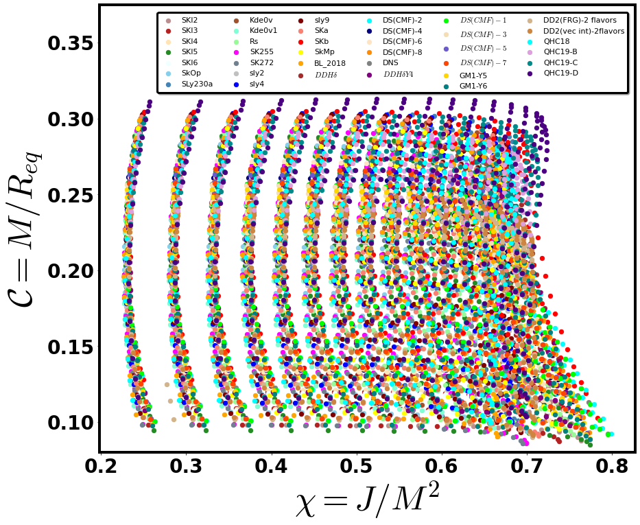
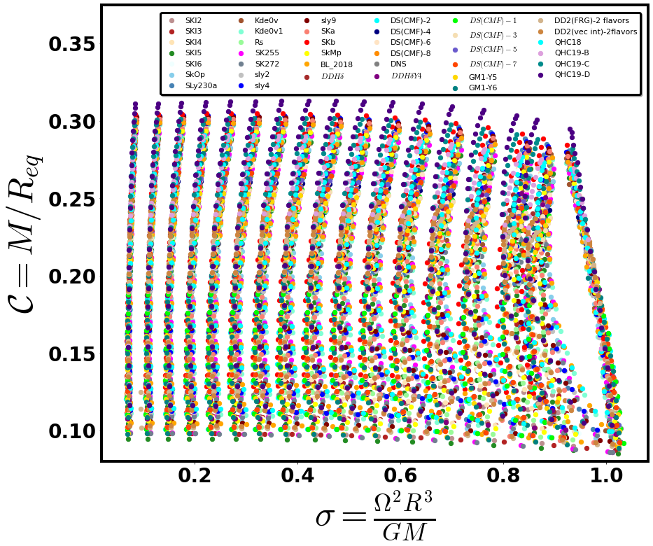
\(C-\chi\) and \(C-\sigma\) representations#
stellar_parameters_plot(eos_data,x='x',y = 'C',y_min = 0.080,y_max=0.375,x_label = r'$\chi=J/M^2 $',
                        y_label = r"$\mathcal{C}=M/R_{eq}$",n_col=6,border_axes=1)
stellar_parameters_plot(eos_data,x='sigma',y = 'C',y_min = 0.080,y_max=0.375,x_label = r'$\sigma=\frac{\Omega^2R^3}{GM} $',
                        y_label = r"$\mathcal{C}=M/R_{eq}$",n_col=6,border_axes=1)
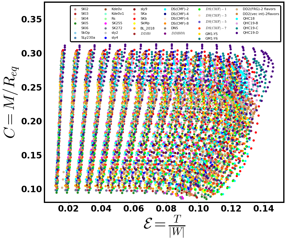
stellar_parameters_plot(eos_data,x='T/W',y = 'C',y_min = 0.080,y_max=0.375,x_label = r'$\mathcal{E}=\frac{T}{|W|}$',
                        y_label = r"$C=M/R_{eq}$",n_col=6,border_axes=1)
Investigation of the \(\bar{Q}=\bar{Q}(C,\sigma)\) parameterization#
d = {'C': C,'x':x_spin ,'sigma': sigma,'q':quadr}
df=pd.DataFrame(data=d, index=None, columns=None, dtype=None, copy=False)
df.reset_index(drop=True, inplace=True)
#df
Cross validation statistical metrics and results for different ‘pol degrees’ \(\kappa\)#
#cv_results = c_val_performace_results_for_k(df,x='C',y='sigma',z='q')
#cv_results
pd.read_csv(r"LOOCV_results/q_c_sigma_cv_scores.txt", sep=' ')
| MAE | Max_Error | MSE | d(%) | MAPE(%) | Explained_Variance | k | |
|---|---|---|---|---|---|---|---|
| 0 | 0.226500 | 2.549192 | 0.089604 | 81.852650 | 7.320705 | 1.0 | 2.0 |
| 1 | 0.091827 | 1.093373 | 0.017452 | 36.463143 | 2.689447 | 1.0 | 3.0 |
| 2 | 0.065704 | 0.771295 | 0.010369 | 13.010768 | 1.585024 | 1.0 | 4.0 |
| 3 | 0.063222 | 0.744127 | 0.009745 | 6.899128 | 1.490653 | 1.0 | 5.0 |
| 4 | 0.064941 | 0.787547 | 0.009940 | 9.552421 | 1.575541 | 1.0 | 6.0 |
| 5 | 0.062111 | 0.757730 | 0.009515 | 7.172604 | 1.455118 | 1.0 | 7.0 |
# best functional form form for pol_degree = 5
Linear Regression at training data#
df['qbar_model'] = Regression_function(df,x = 'C',y= 'sigma' ,z='q', pol_degree=5, x_power = 'C',y_power='sigma')[0]
#df['qbar_model']
\(R^2\) - quality index#
Regression_function(df,x = 'C',y= 'sigma' ,z='q', pol_degree=5, x_power = 'C',y_power='sigma')[1]
0.9983896849623227
Evaluation functions at training data#
relative_training_error_plot(df, 'q' , 'qbar_model', xlabel='Data',
                             ylabel=r'$(\Delta\bar{Q}/\bar{Q})\times 100\%$') #,fig_title = 'test.png'
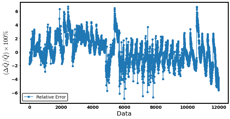
<AxesSubplot:xlabel='Data', ylabel='$(\\Delta\\bar{Q}/\\bar{Q})\\times 100\\%$'>
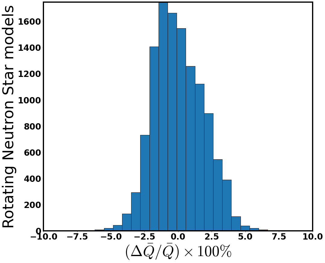
training_error_funct(df, 'q' , 'qbar_model')
| train_Max_Error | d_max_training(%) | MAPE_taining(%) | |
|---|---|---|---|
| 0 | 0.738374 | 6.866255 | 1.487652 |
training_relative_error_hist(df, 'q', 'qbar_model',
                             r'$(\Delta\bar{Q}/\bar{Q})\times 100\%$', r'Rotating Neutron Star models',n_bins=20,
                             x1_lim=-10, x2_lim=10)
Error distribution at space#
relative_error_space_distribution(df, 'C' , 'sigma' ,'q','qbar_model' ,
                                  '$C$','$\sigma$', r'$(|\Delta\bar{Q}|/\bar{Q})\times 100\%$',
                                  view2=240)
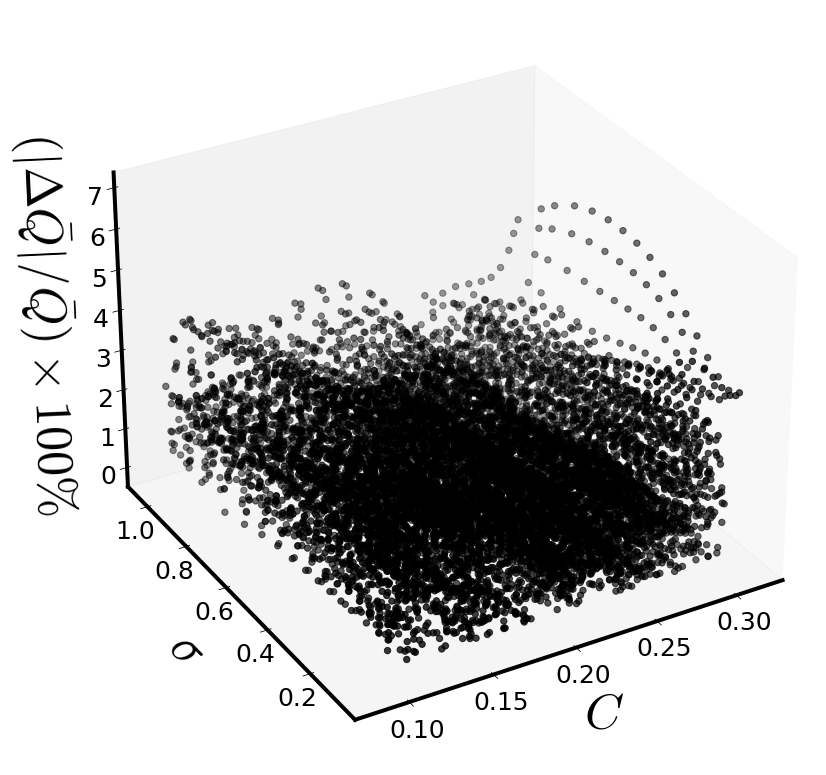
Considerable relative deviations#
#variance_of_errors(df=df,reference_deviation = 5,z = df['q'],z_model=df['qbar_model'])
#(variance_of_errors(df=df,reference_deviation = 5,z = df['q'],z_model=df['qbar_model'])[['C','sigma']][:48])
#(variance_of_errors(df=df,reference_deviation = 5,z = df['q'],z_model=df['qbar_model'])[['C','sigma']][48:])
#(variance_of_errors(df=df,reference_deviation = 5,z = df['q'],z_model=df['qbar_model'])[['C','sigma']]).max()
Best Model’s optimizers-coefficients#
# model's intercept
a_00 = Regression_function(df,x = 'C',y= 'sigma' ,z='q', pol_degree=5, x_power = 'C',y_power='sigma')[2]

# model's other coefficients
a_nm = Regression_function(df,x = 'C',y= 'sigma' ,z='q', pol_degree=5, x_power = 'C',y_power='sigma')[3]

# a_nm stored to data frame
coef=pd.DataFrame(a_nm,columns=["coef"])
# coefficient combinations
test = Regression_function(df,x = 'C',y= 'sigma' ,z='q', pol_degree=5, x_power = 'C',y_power='sigma')[4]
#test
powers = Regression_function(df,x = 'C',y= 'sigma' ,z='q',
                            pol_degree=5, x_power = 'C',y_power='sigma')[5]
#powers
def q_bar_funct(C,sigma):
    results=0
    for i in range(0,len(powers)):
        results+=(coef["coef"][i]*C**(powers["C"][i])*sigma**(powers["sigma"][i]))

    return a_00 + results
Regression Function#
q_bar_funct(C_s,sigma_s)
\[\displaystyle - 50058.6671887959 \mathcal{C}^{5} - 5186.19270734206 \mathcal{C}^{4} \sigma + 61273.0850581345 \mathcal{C}^{4} - 604.254218115162 \mathcal{C}^{3} \sigma^{2} + 5564.52593040181 \mathcal{C}^{3} \sigma - 30342.8560570677 \mathcal{C}^{3} - 93.5686038633851 \mathcal{C}^{2} \sigma^{3} + 618.572725383674 \mathcal{C}^{2} \sigma^{2} - 2387.15128458972 \mathcal{C}^{2} \sigma + 7768.1018162227 \mathcal{C}^{2} - 13.503802917148 \mathcal{C} \sigma^{4} + 76.9653211797515 \mathcal{C} \sigma^{3} - 225.548462084009 \mathcal{C} \sigma^{2} + 500.949544887105 \mathcal{C} \sigma - 1069.90020498716 \mathcal{C} + 1.44555400224044 \sigma^{5} - 0.096154369815387 \sigma^{4} - 10.9551318374866 \sigma^{3} + 27.1374820754294 \sigma^{2} - 43.9930955035481 \sigma + 68.0275059789124\]
Indicative Curve fits#
Yagi and Yunes universal relations for slowly rotating NSs#
def q_c_YY(x):
    q = -0.2588/x + 0.2274/(x**2) + 0.0009528/(x**3) - 0.0007747/(x**4)
    return q
sigma_values = np.arange(0.01,0.1,0.01)
C_values = np.arange(0.09,0.29,0.02)
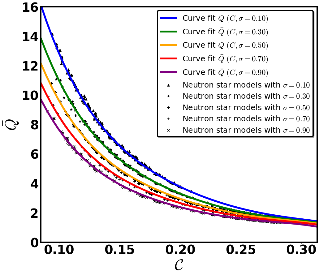
Q_bar_model_curve_fits(df, 'C',y = sigma_values, xlabel=r'$C $', ylabel=r"$\bar{Q}$", fig_label = r'$\sigma$')
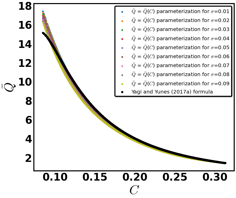
Model Chareacteristic curves parameterized for different values of \(\sigma\) in to comparison to data points#
df_sigma_0_1=df[(df['sigma']>0.095) & (df['sigma']<=0.11)].copy()
df_sigma_0_1.reset_index(drop=True, inplace=True)

df_sigma_0_3=df[(df['sigma']>0.295) & (df['sigma']<=0.327)].copy()
df_sigma_0_3.reset_index(drop=True, inplace=True)

df_sigma_0_5=df[(df['sigma']>0.49) & (df['sigma']<=0.5037)].copy()
df_sigma_0_5.reset_index(drop=True, inplace=True)

df_sigma_0_7=df[(df['sigma']>0.69) & (df['sigma']<=0.705)].copy()
df_sigma_0_7.reset_index(drop=True, inplace=True)

df_sigma_0_9=df[(df['sigma']>0.885) & (df['sigma']<=0.9049)].copy()
df_sigma_0_9.reset_index(drop=True, inplace=True)

#------------------------------------------------
df_sigma_data = [df_sigma_0_1, df_sigma_0_3, df_sigma_0_5, df_sigma_0_7,df_sigma_0_9]
#------------------------------------------------
c_data = np.linspace(df['C'].min(), df['C'].max(),50)
q_data = np.linspace(df['q'].min(), df['q'].max(),50)
def Qbar_curve_fits_compared_to_sigma_data(data_list, x,z, x_data, z_data, xlabel,zlabel):

    markers = ["^", "*", "P", "+", "x"]
    sigma = np.arange(0.1,1.1,0.2)
    color2 = ["blue","green","orange","red","purple"]

    #plt.figure(figsize=(16, 14))
    fig,ax = plt.subplots(figsize=(16, 14),)
    labels_text_size = 50

    scatter_size = 55

    plt.xticks(fontsize=40, fontweight="bold")
    plt.yticks(fontsize=40, fontweight="bold")
    plt.xlabel(xlabel,size=labels_text_size )
    plt.ylabel(zlabel,size=labels_text_size )

    for i in range(0,len(data_list)):

        plt.plot((x_data),(q_bar_funct(x_data,sigma[i])),color=color2[i], lw = 6,
                    label = f"Curve fit {zlabel} $(C,\sigma={sigma[i]:0.2f})$" )

        plt.scatter((data_list[i][x]),(data_list[i][z]),color='black',s=scatter_size,
                    marker=markers[i] ,label = f"Neutron star models with $\sigma={sigma[i]:0.2f}$")

    plt.xlim(x_data.min(),x_data.max())
    plt.ylim(0,16)
    leg = plt.legend(loc="best", prop={'size': 25}, shadow=True, fontsize="large", ncol = 1)

    leg.get_frame().set_linewidth(4.0)
    leg.get_frame().set_edgecolor('black')


    for axis in ['top','bottom','left','right']:
        ax.spines[axis].set_linewidth(4.0)


    plt.grid(False)

    #plt.savefig('q_c_sigma_fixed.png',dpi=100,facecolor="w",bbox_inches='tight',transparent=True, pad_inches=0.2)
    plt.show()
Qbar_curve_fits_compared_to_sigma_data(df_sigma_data, 'C','q', x_data =c_data,
                                       z_data=q_data, xlabel = r'$\mathcal{C}$',zlabel = r'$\bar{Q}$')
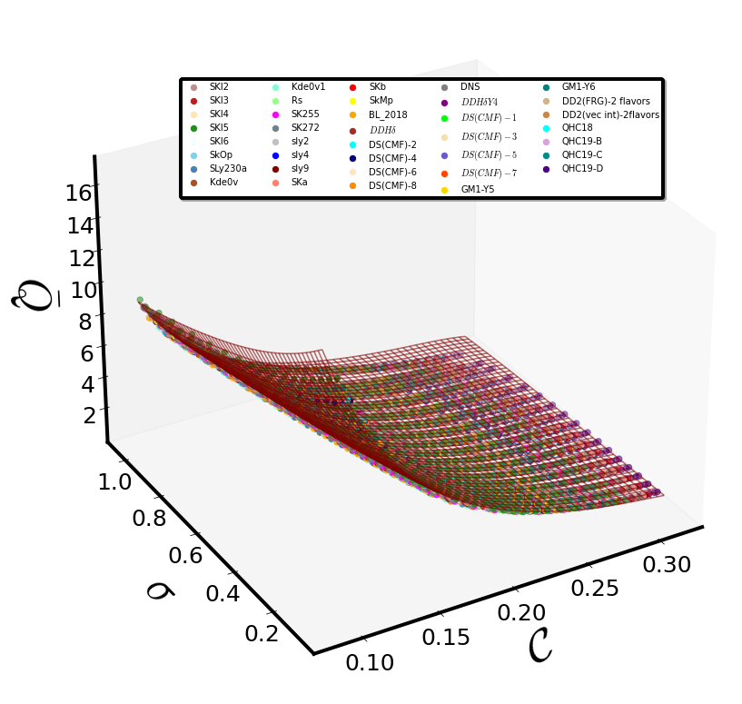
Fitting Surface compared to data#
x1 = mesh_grid_funct(df,x_name = 'C', y_name = 'sigma')[0]
y1 = mesh_grid_funct(df,x_name = 'C', y_name = 'sigma')[1]
Z = q_bar_funct(x1,y1)
Surface_plot_funct_2(eos_data, 'C','sigma','q_tilde_GH', xlabel=r'$\mathcal{C}$',ylabel='$\sigma$',zlabel=r'$\bar{Q}$',
                     view2=240, n_col=5, border_axes=8, X=x1,Y=y1,Z=Z, l_w=1.5)
Investigation of the \(\frac{R_{eq}}{M} = \mathcal{K}(\chi,\bar{Q})\) parameterization#
df_a = {'C':C_2,'K':RoverM_2,'x': x_spin_2,'qbar': quadr_2, 'ln(qbar)':ln_Qbar_2}
df_a = pd.DataFrame(data=df_a, index=None, columns=None, dtype=None, copy=False)
df_a.reset_index(drop=True, inplace=True)
#dfa
Cross validation statistical metrics and results for different ‘pol degrees’ \(\kappa\)#
#cv_results = c_val_performace_results_for_k(df_a,x='x',y='qbar',z='K')
#cv_results
pd.read_csv(r"LOOCV_results/K_chi_Qbar_cv_scores.txt", sep=' ')
| MAE | Max_Error | MSE | d(%) | MAPE(%) | Explained_Variance | k | |
|---|---|---|---|---|---|---|---|
| 0 | 0.088139 | 0.708150 | 0.014852 | 11.919031 | 1.582944 | 1.0 | 2.0 |
| 1 | 0.076927 | 0.707428 | 0.011816 | 7.190012 | 1.329090 | 1.0 | 3.0 |
| 2 | 0.072480 | 0.681883 | 0.010886 | 6.930379 | 1.221118 | 1.0 | 4.0 |
| 3 | 0.070473 | 0.637602 | 0.010521 | 6.480330 | 1.177226 | 1.0 | 5.0 |
| 4 | 0.087054 | 0.992615 | 0.015122 | 9.374081 | 1.487484 | 1.0 | 6.0 |
| 5 | 0.070271 | 0.618097 | 0.010511 | 6.687497 | 1.179050 | 1.0 | 7.0 |
# best functional form form for pol_degree = 5
Linear Regression at training data#
df_a['K_model'] = Regression_function(df_a,x = 'x',y= 'qbar' ,z='K', pol_degree=5, x_power = 'x',y_power='Qbar')[0]
#df_a['K_model']
\(R^2\) - quality index#
Regression_function(df_a,x = 'x',y= 'qbar' ,z='K', pol_degree=5, x_power = 'x',y_power='Qbar')[1]
0.9967495025538458
Evaluation functions at training data#
relative_training_error_plot(df_a, 'K' , 'K_model', xlabel='Data', ylabel=r'$(\Delta\mathcal{K}/\mathcal{K})\times 100\%$')
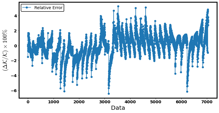
<AxesSubplot:xlabel='Data', ylabel='$(\\Delta\\mathcal{K}/\\mathcal{K})\\times 100\\%$'>
training_error_funct(df_a, 'K' , 'K_model')
| train_Max_Error | d_max_training(%) | MAPE_taining(%) | |
|---|---|---|---|
| 0 | 0.633994 | 6.443663 | 1.173426 |
training_relative_error_hist(df_a, 'K', 'K_model',
                             r'$(\Delta\mathcal{K}/\mathcal{K})\times 100\%$', r'Rotating Neutron Star models',n_bins = 20,
                             x1_lim=-10, x2_lim=10)
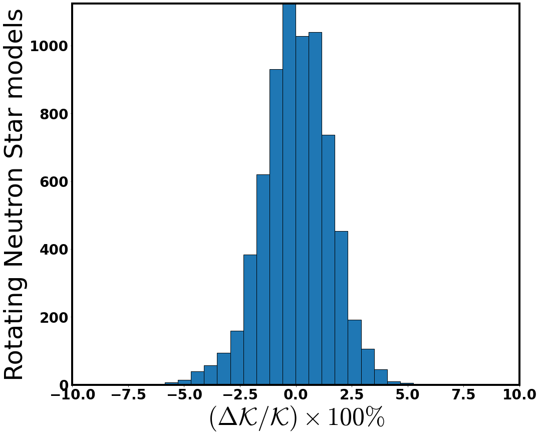
Error distribution at space#
relative_error_space_distribution(df_a, 'x' , 'qbar' ,'K','K_model' ,
                                  r'$\chi$',r'$\bar{Q}$', r'$(|\Delta\mathcal{K}|/\mathcal{K})\times 100\%$',
                                  view2=220)
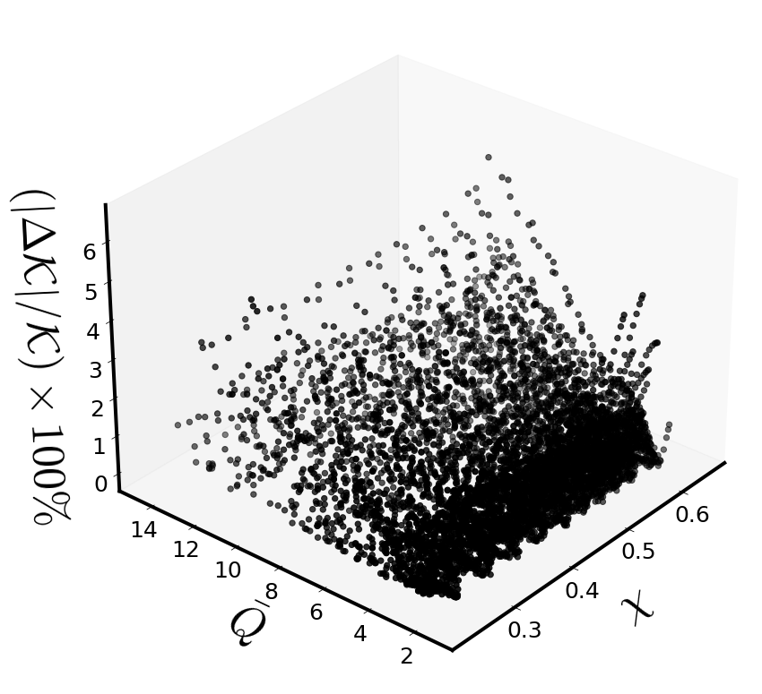
Cosiderable relative deviations#
variance_of_errors(df=df_a,reference_deviation = 5,z = df_a['K'],z_model=df_a['K_model'])[['x','C','qbar']].min()
x       0.248295
C       0.095602
qbar    6.458684
dtype: float64
variance_of_errors(df=df_a,reference_deviation = 5,z = df_a['K'],z_model=df_a['K_model'])[['x','C','qbar']].max()
x        0.602231
C        0.124325
qbar    10.564225
dtype: float64
len(variance_of_errors(df=df_a,reference_deviation = 5,z = df_a['K'],z_model=df_a['K_model'])[['x','C','qbar']])
18
Best Model’s optimizers-coefficients#
# model's intercept
a_new_00 = Regression_function(df_a,x = 'x',y= 'qbar' ,z='K', pol_degree=5, x_power = 'x',y_power='Qbar')[2]
# model's other coefficients
a_new_nm = Regression_function(df_a,x = 'x',y= 'qbar' ,z='K', pol_degree=5, x_power = 'x',y_power='Qbar')[3]
#coefficients to data frame
coef_a=pd.DataFrame(a_new_nm,columns=["coef"])
powers_a = Regression_function(df_a,x = 'x',y= 'qbar' ,z='K', pol_degree=5,
                               x_power = 'x',y_power='Qbar')[5]
#powers_a
def K_chi_qbar_funct(x,q):
    results=0
    for i in range(0,len(powers_a)):
        results+=(coef_a["coef"][i]*x**(powers_a["x"][i])*q**(powers_a["Qbar"][i]))

    return a_new_00 + results
Regression Function#
K_chi_qbar_funct(chi_s, qbar_s)
\[\displaystyle - 1244.3347967123 \chi^{5} + 18.2887633011346 \chi^{4} {\left(\bar{Q}\right)} + 2428.50952745328 \chi^{4} + 0.267469754081008 \chi^{3} {\left(\bar{Q}\right)}^{2} - 32.8145138456262 \chi^{3} {\left(\bar{Q}\right)} - 1841.75670236137 \chi^{3} - 0.0122285421139341 \chi^{2} {\left(\bar{Q}\right)}^{3} - 0.158349573402441 \chi^{2} {\left(\bar{Q}\right)}^{2} + 21.3985366813532 \chi^{2} {\left(\bar{Q}\right)} + 677.640400640994 \chi^{2} - 0.000438425543686449 \chi {\left(\bar{Q}\right)}^{4} + 0.0196520597526718 \chi {\left(\bar{Q}\right)}^{3} - 0.117018459003887 \chi {\left(\bar{Q}\right)}^{2} - 4.94610324454508 \chi {\left(\bar{Q}\right)} - 121.682754597622 \chi + 4.95022681974433 \cdot 10^{-5} {\left(\bar{Q}\right)}^{5} - 0.00193982406006728 {\left(\bar{Q}\right)}^{4} + 0.0279493080650313 {\left(\bar{Q}\right)}^{3} - 0.209569019615312 {\left(\bar{Q}\right)}^{2} + 1.82381657525581 {\left(\bar{Q}\right)} + 10.0965916959039\]
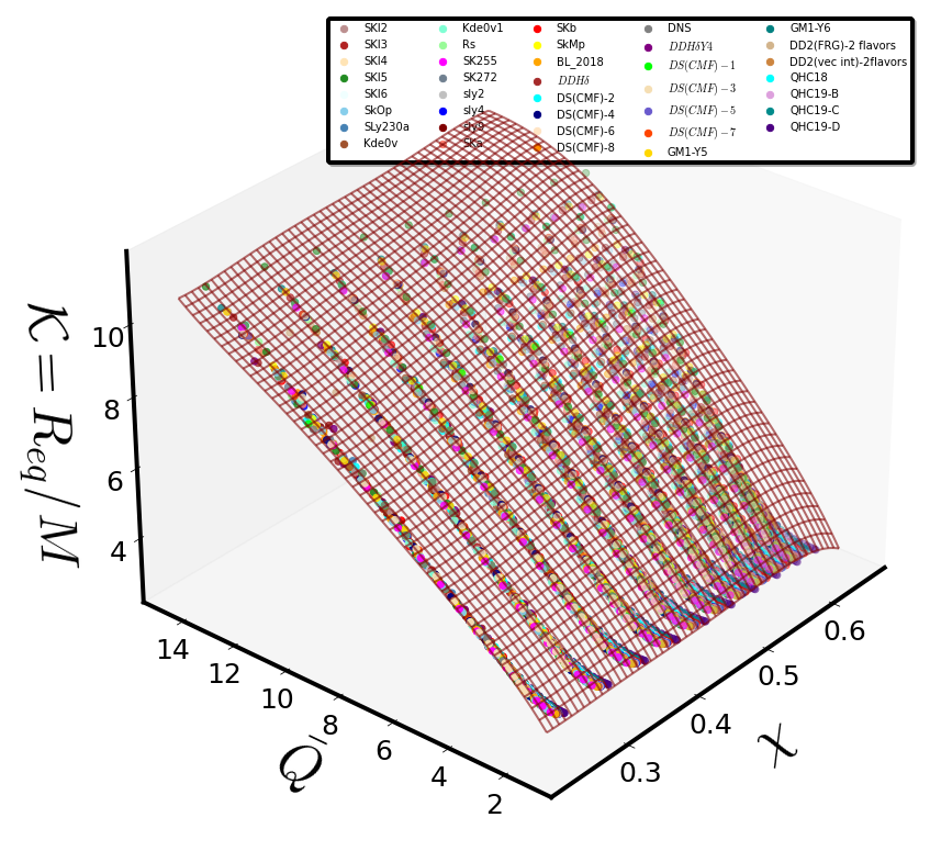
Fitting Surface compared to data#
x1_a = mesh_grid_funct(df_a,x_name = 'x', y_name = 'qbar')[0]
y1_a = mesh_grid_funct(df_a,x_name = 'x', y_name = 'qbar')[1]

Z_a = K_chi_qbar_funct(x1_a,y1_a)
Surface_plot_funct_2(eos_data2, 'x','q_tilde_GH','R/M', xlabel=r'$\chi$',ylabel=r'$\bar{Q}$',zlabel=r'$\mathcal{K}=R_{eq}/M$',
                     view2=220, n_col=5, border_axes=1, X=x1_a,Y=y1_a,Z=Z_a, l_w=2.0)
Investigation of the \(\frac{T}{|W|}=\mathcal{E}\left(\chi,\ln(\bar{Q})\right)\) parameterization#
df_b = {'C':C_2,'x': x_spin_2,'qbar':quadr_2,'ln(qbar)':ln_Qbar_2, 'T/W': T_over_W_2}
df_b = pd.DataFrame(data=df_b, index=None, columns=None, dtype=None, copy=False)
df_b.reset_index(drop=True, inplace=True)
#df_b
Cross validation statistical metrics and results for different ‘pol degrees’ \(\kappa\)#
#cv_results = c_val_performace_results_for_k(df_b,x='x',y='ln(qbar)',z='T/W')
#cv_results
pd.read_csv(r"LOOCV_results/T_W_chi_lnQbar_cv_scores.txt", sep=' ')
# best functional form form for pol_degree = 5
| MAE | Max_Error | MSE | d(%) | MAPE(%) | Explained_Variance | k | |
|---|---|---|---|---|---|---|---|
| 0 | 0.000713 | 0.004060 | 9.208962e-07 | 23.377261 | 2.089047 | 1.0 | 2.0 |
| 1 | 0.000232 | 0.001815 | 1.092455e-07 | 11.888116 | 0.607645 | 1.0 | 3.0 |
| 2 | 0.000151 | 0.001576 | 5.911629e-08 | 5.432689 | 0.324699 | 1.0 | 4.0 |
| 3 | 0.000134 | 0.001475 | 5.269914e-08 | 3.019543 | 0.268789 | 1.0 | 5.0 |
| 4 | 0.000131 | 0.001518 | 5.075441e-08 | 2.361797 | 0.258584 | 1.0 | 6.0 |
| 5 | 0.000129 | 0.001537 | 4.966900e-08 | 2.091604 | 0.256437 | 1.0 | 7.0 |
Linear Regression at training data#
df_b['E_model'] = Regression_function(df_b,x = 'x',y= 'ln(qbar)' ,z='T/W', pol_degree=5, x_power = 'x',y_power='lnQbar')[0]
#df_b['E_model']
\(R^2\) - quality index#
Regression_function(df_b,x = 'x',y= 'ln(qbar)' ,z='T/W', pol_degree=5, x_power = 'x',y_power='lnQbar')[1]
0.9998990143432449
Evaluation functions at training data#
relative_training_error_plot(df_b, 'T/W' , 'E_model', xlabel='Data', ylabel=r'$(\Delta\mathcal{E}/\mathcal{E})\times 100\%$')
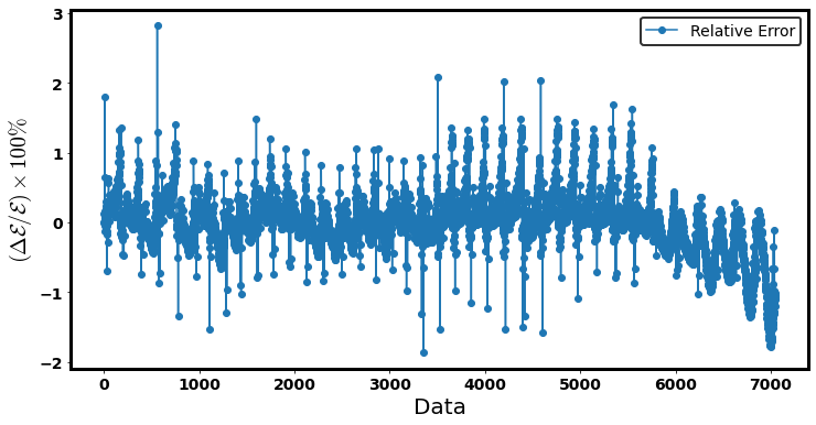
<AxesSubplot:xlabel='Data', ylabel='$(\\Delta\\mathcal{E}/\\mathcal{E})\\times 100\\%$'>
training_error_funct(df_b, 'T/W' , 'E_model')
| train_Max_Error | d_max_training(%) | MAPE_taining(%) | |
|---|---|---|---|
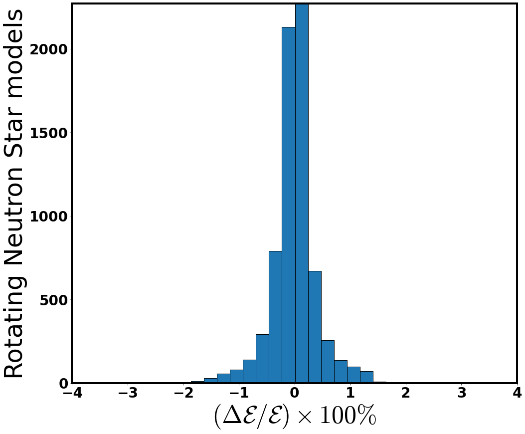
| 0 | 0.00147 | 2.815006 | 0.267855 |
training_relative_error_hist(df_b, 'T/W', 'E_model',
                             r'$(\Delta\mathcal{E}/\mathcal{E})\times 100\%$', r'Rotating Neutron Star models',n_bins = 20,
                             x1_lim=-4, x2_lim=4)
Error distribution at space#
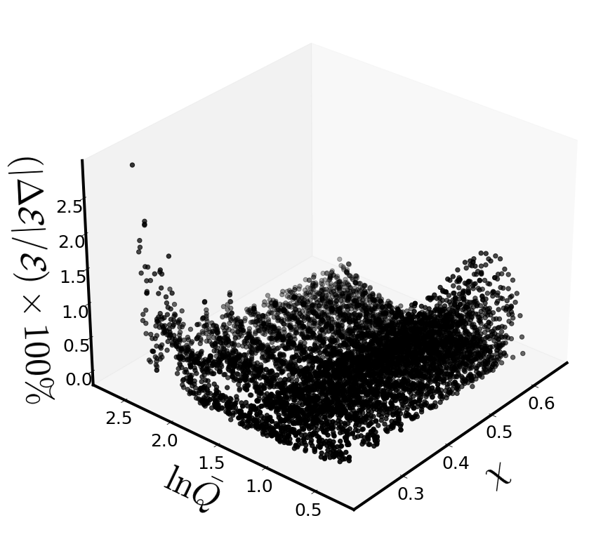
relative_error_space_distribution(df_b, 'x' , 'ln(qbar)' ,'T/W','E_model' ,
                                  r'$\chi$',r'$\ln\bar{Q}$', r'$(|\Delta\mathcal{E}|/\mathcal{E})\times 100\%$',
                                  view2=220)
Considerable relative deviations#
#variance_of_errors(df=df_b,reference_deviation = 1.5,z = df_b['T/W'],z_model=df_b['E_model'])[['x','C','qbar']]
len(variance_of_errors(df=df_b,reference_deviation = 1.5,z = df_b['T/W'],z_model=df_b['E_model'])[['x','C','qbar']])
35
variance_of_errors(df=df_b,reference_deviation = 1.5,z = df_b['T/W'],z_model=df_b['E_model'])[['x','C','qbar']].min()
x       0.242129
C       0.094434
qbar    1.436349
dtype: float64
variance_of_errors(df=df_b,reference_deviation = 1.5,z = df_b['T/W'],z_model=df_b['E_model'])[['x','C','qbar']].max()
x        0.576881
C        0.306934
qbar    14.602864
dtype: float64
Best Model’s optimizers-coefficients#
#model's intercept
a_new2_00 = Regression_function(df_b,x = 'x',y= 'ln(qbar)' ,z='T/W', pol_degree=5, x_power = 'x',y_power='lnQbar')[2]
# Other coefficients
a_new2_nm = Regression_function(df_b,x = 'x',y= 'ln(qbar)' ,z='T/W', pol_degree=5, x_power = 'x',y_power='lnQbar')[3]
# results stored to data frame
coef_b=pd.DataFrame(a_new2_nm,columns=["coef"])
powers_b = Regression_function(df_b,x = 'x',y= 'ln(qbar)' ,z='T/W', pol_degree=5, x_power = 'x',y_power='lnQbar')[5]
#powers_b
def E_chi_lnQbar_funct(x,lnq):
    results=0
    for i in range(0,len(powers_b)):
        results+=(coef_b["coef"][i]*x**(powers_b["x"][i])*lnq**(powers_b["lnQbar"][i]))

    return a_new2_00 + results
Regression Function#
E_chi_lnQbar_funct(chi_s,lnQbar_s)
\[\displaystyle 2.35602089109591 \chi^{5} - 0.447970491423178 \chi^{4} \left(\ln{\bar{Q}}\right) - 4.1338397049757 \chi^{4} + 0.0833530421638261 \chi^{3} \left(\ln{\bar{Q}}\right)^{2} + 0.423709394128891 \chi^{3} \left(\ln{\bar{Q}}\right) + 2.89427031873595 \chi^{3} + 0.00539876822696325 \chi^{2} \left(\ln{\bar{Q}}\right)^{3} - 0.112825660764877 \chi^{2} \left(\ln{\bar{Q}}\right)^{2} - 0.1480055050144 \chi^{2} \left(\ln{\bar{Q}}\right) - 0.706683559434699 \chi^{2} - 0.00435015261782149 \chi \left(\ln{\bar{Q}}\right)^{4} + 0.0287830119285485 \chi \left(\ln{\bar{Q}}\right)^{3} - 0.0496044527457874 \chi \left(\ln{\bar{Q}}\right)^{2} + 0.117315009245361 \chi \left(\ln{\bar{Q}}\right) + 0.129590008212152 \chi + 0.000517876822173371 \left(\ln{\bar{Q}}\right)^{5} - 0.0027620776855964 \left(\ln{\bar{Q}}\right)^{4} + 0.00385838510266808 \left(\ln{\bar{Q}}\right)^{3} - 0.000567663174628646 \left(\ln{\bar{Q}}\right)^{2} - 0.00951385767132625 \left(\ln{\bar{Q}}\right) - 0.00697861553093789\]
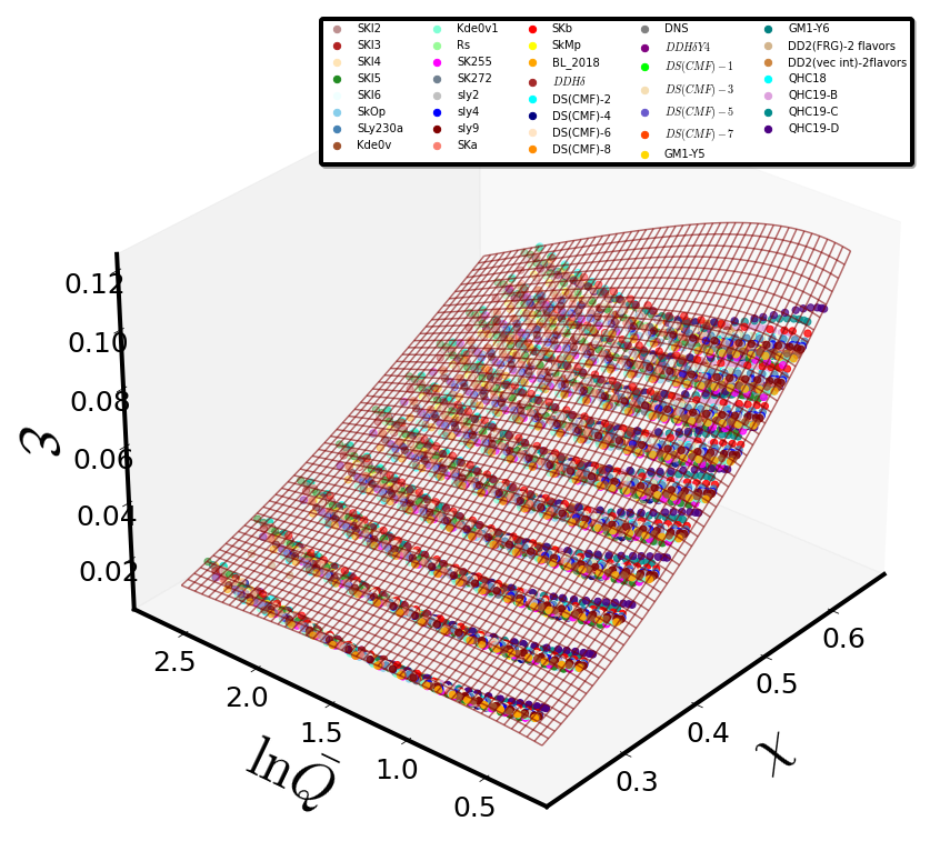
Fitting Surface compared to data#
x1_b = mesh_grid_funct(df_b,x_name = 'x', y_name = 'ln(qbar)')[0]
y1_b = mesh_grid_funct(df_b,x_name = 'x', y_name = 'ln(qbar)')[1]
Z_b = E_chi_lnQbar_funct(x1_b,y1_b)
Surface_plot_funct_2(eos_data2, 'x','ln(qbar)','T/W', xlabel=r'$\chi$',ylabel=r'$\ln\bar{Q}$',zlabel=r'$\mathcal{E}$',
                     view2=220, n_col=5, border_axes=1, X=x1_b,Y=y1_b,Z=Z_b, l_w=1.5)
Investigation of the \(\mathcal{D}=\frac{M\times \tilde{f}}{\chi} = F (\chi,\ln\bar{Q})\) parameterization#
df_c = {'C':C_2,'x': x_spin_2,'sigma':sigma_2,"f(kHz)":f_kHz_2,'qbar': quadr_2,'lnQbar':np.log(quadr_2),'M*f/x':M_f_over_x_2}
df_c = pd.DataFrame(data=df_c, index=None, columns=None, dtype=None, copy=False)
df_c.reset_index(drop=True, inplace=True)
#df_c
Cross validation statistical metrics and results for different ‘pol degrees’ \(\kappa\)#
#cv_results =c_val_performace_results_for_k(df_c,x='x',y='lnQbar',z='M*f/x')
#cv_results
pd.read_csv(r"LOOCV_results/D_chi_lnQbar_cv_scores.txt", sep=' ')
# best functional form form for pol_degree = 4
| MAE | Max_Error | MSE | d(%) | MAPE(%) | Explained_Variance | k | |
|---|---|---|---|---|---|---|---|
| 0 | 0.000192 | 0.001352 | 6.467440e-08 | 25.341231 | 1.350909 | 1.0 | 2.0 |
| 1 | 0.000082 | 0.000638 | 1.229733e-08 | 13.544633 | 0.532285 | 1.0 | 3.0 |
| 2 | 0.000057 | 0.000439 | 6.666853e-09 | 5.306419 | 0.322180 | 1.0 | 4.0 |
| 3 | 0.000054 | 0.000407 | 6.169108e-09 | 5.633763 | 0.297211 | 1.0 | 5.0 |
| 4 | 0.000053 | 0.000412 | 6.053958e-09 | 5.348801 | 0.290430 | 1.0 | 6.0 |
| 5 | 0.000053 | 0.000398 | 5.927809e-09 | 4.969797 | 0.296948 | 1.0 | 7.0 |
Linear Regression at training data#
df_c['Mf/x_model'] = Regression_function(df_c,x = 'x',y= 'lnQbar' ,z='M*f/x', pol_degree=4, x_power = 'x',y_power='lnQbar')[0]
#df_c['Mf/x_model']
\(R^2\) - quality index#
Regression_function(df_c,x = 'x',y= 'lnQbar' ,z='M*f/x', pol_degree=4, x_power = 'x',y_power='lnQbar')[1]
0.9998855421883416
Evaluation functions at training data#
relative_training_error_plot(df_c, 'M*f/x' , 'Mf/x_model', xlabel='Data', ylabel=r'$(\Delta\mathcal{D}/\mathcal{D})\times 100\%$')
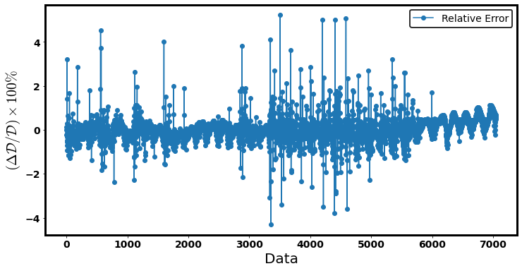
<AxesSubplot:xlabel='Data', ylabel='$(\\Delta\\mathcal{D}/\\mathcal{D})\\times 100\\%$'>
training_error_funct(df_c, 'M*f/x' , 'Mf/x_model')
| train_Max_Error | d_max_training(%) | MAPE_taining(%) | |
|---|---|---|---|
| 0 | 0.000438 | 5.219764 | 0.321251 |
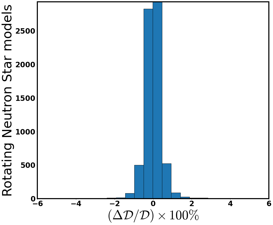
training_relative_error_hist(df_c, 'M*f/x', 'Mf/x_model',
                             r'$(\Delta\mathcal{D}/\mathcal{D})\times 100\%$', r'Rotating Neutron Star models',n_bins = 20,
                             x1_lim=-6, x2_lim=6)
Error distribution at space#
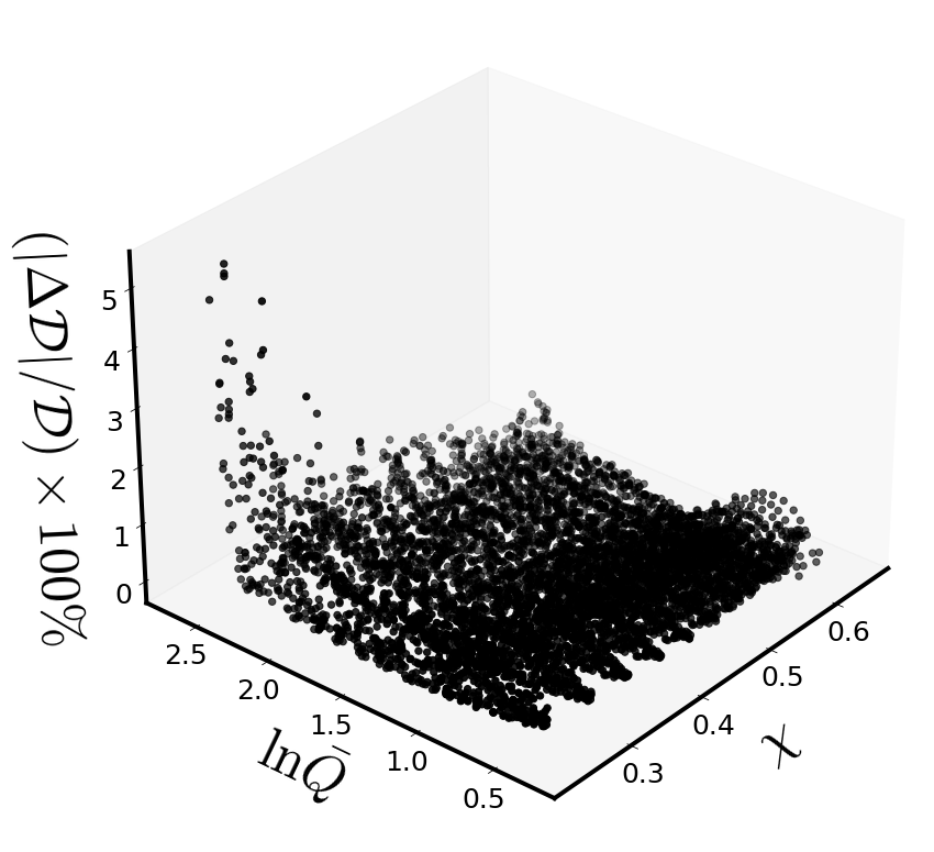
relative_error_space_distribution(df_c, 'x' , 'lnQbar' ,'M*f/x','Mf/x_model' ,
                                  r'$\chi$',r'$\ln\bar{Q}$', r'$(|\Delta\mathcal{D}|/\mathcal{D})\times 100\%$',
                                  view2=220)
Considerable relative deviations#
#variance_of_errors(df=df_c,reference_deviation = 2,z = df_c['M*f/x'],z_model=df_c['Mf/x_model'])[['x','C','qbar']]
len(variance_of_errors(df=df_c,reference_deviation = 2,z = df_c['M*f/x'],z_model=df_c['Mf/x_model'])[['x','C','qbar']]
)
42
variance_of_errors(df=df_c,reference_deviation = 2,z = df_c['M*f/x'],z_model=df_c['Mf/x_model'])[['x','C','qbar']].min()
x       0.232810
C       0.094434
qbar    3.329590
dtype: float64
variance_of_errors(df=df_c,reference_deviation = 2,z = df_c['M*f/x'],z_model=df_c['Mf/x_model'])[['x','C','qbar']].max()
x        0.301276
C        0.211560
qbar    14.602864
dtype: float64
Best Model’s optimizers-coefficients#
# model's intercept
a_new3_00 = Regression_function(df_c,x = 'x',y= 'lnQbar' ,z='M*f/x', pol_degree=4, x_power = 'x',y_power='lnQbar')[2]
# Other coefficients
a_new3_nm = Regression_function(df_c,x = 'x',y= 'lnQbar' ,z='M*f/x', pol_degree=4, x_power = 'x',y_power='lnQbar')[3]
# results stored to dataframe
coef_c=pd.DataFrame(a_new3_nm,columns=["coef"])
powers_c = Regression_function(df_c,x = 'x',y= 'lnQbar' ,z='M*f/x', pol_degree=4, x_power = 'x',y_power='lnQbar')[5]
#powers_c
def Mf_over_x_chi_lnQbar_funct(x,lnq):
    results=0
    for i in range(0,len(powers_c)):
        results+=(coef_c["coef"][i]*x**(powers_c["x"][i])*lnq**(powers_c["lnQbar"][i]))

    return a_new3_00 + results
Regression Function#
Mf_over_x_chi_lnQbar_funct(chi_s,lnQbar_s)
\[\displaystyle - 0.0147728500634506 \chi^{4} + 0.00752116861991202 \chi^{3} \left(\ln{\bar{Q}}\right) + 0.0140392142928143 \chi^{3} + 0.0034932330415095 \chi^{2} \left(\ln{\bar{Q}}\right)^{2} - 0.0175793547611627 \chi^{2} \left(\ln{\bar{Q}}\right) - 0.00276192265198208 \chi^{2} - 0.00262258358299214 \chi \left(\ln{\bar{Q}}\right)^{3} + 0.011903211319849 \chi \left(\ln{\bar{Q}}\right)^{2} - 0.0127773194000064 \chi \left(\ln{\bar{Q}}\right) + 0.00251191105289285 \chi + 0.000322310427167579 \left(\ln{\bar{Q}}\right)^{4} - 0.00152187660421336 \left(\ln{\bar{Q}}\right)^{3} + 0.00505813198005616 \left(\ln{\bar{Q}}\right)^{2} - 0.0219273871982111 \left(\ln{\bar{Q}}\right) + 0.0403032600466225\]
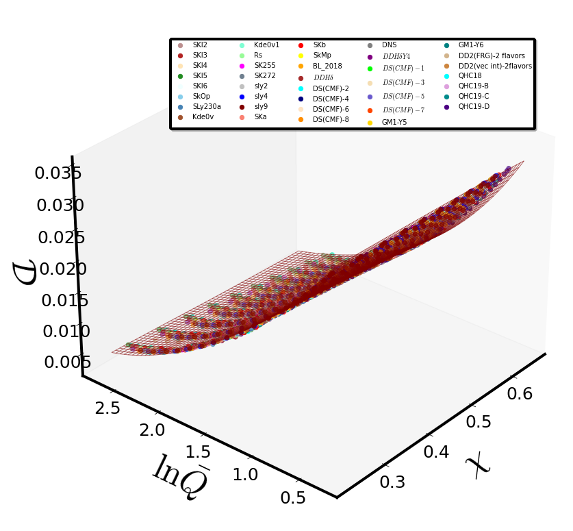
Fitting Surface compared to data#
x1_c = mesh_grid_funct(df_c,x_name = 'x', y_name = 'lnQbar')[0]
y1_c = mesh_grid_funct(df_c,x_name = 'x', y_name = 'lnQbar')[1]
Z_c = Mf_over_x_chi_lnQbar_funct(x1_c,y1_c)
Surface_plot_funct_2(eos_data2, 'x','ln(qbar)','M*f/x', xlabel=r'$\chi$',ylabel=r'$\ln\bar{Q}$',
                     zlabel=r'$\mathcal{D}$',
                     view2=220, n_col=5, border_axes=5, X=x1_c,Y=y1_c,Z=Z_c, l_w=1.)
———————————————————————————————#
Investigation of the \(\bar{I}=f(\chi,\bar{Q})\) parameterization#
df2 = {'C':C,'K':C**(-1),'f(kHz)': f_kHz,'x': x_spin,'sigma':sigma,'qbar': quadr, "ln(qbar)":np.log(quadr),'Ibar':I_bar,
       'Mf/x':M_km_f_kHz_over_x}
df2=pd.DataFrame(data=df2, index=None, columns=None, dtype=None, copy=False)
df2.reset_index(drop=True, inplace=True)
Cross validation statistical metrics and results for different ‘pol degrees’ \(\kappa\)#
#cv_results = c_val_performace_results_for_k(df2,x='x',y='qbar',z='Ibar')
#cv_results
pd.read_csv(r"LOOCV_results/Ibar_chi_Qbar_cv_scores.txt", sep=' ')
# best functional form for pol_degree = 4
| MAE | Max_Error | MSE | d(%) | MAPE(%) | Explained_Variance | k | |
|---|---|---|---|---|---|---|---|
| 0 | 0.109743 | 1.808035 | 0.022264 | 11.319820 | 1.204714 | 1.0 | 2.0 |
| 1 | 0.047923 | 1.604626 | 0.005447 | 5.919222 | 0.524404 | 1.0 | 3.0 |
| 2 | 0.034614 | 1.521632 | 0.003759 | 5.613070 | 0.359616 | 1.0 | 4.0 |
| 3 | 0.031042 | 1.481650 | 0.003366 | 5.465580 | 0.311196 | 1.0 | 5.0 |
| 4 | 0.029576 | 1.587927 | 0.003213 | 5.857621 | 0.293900 | 1.0 | 6.0 |
| 5 | 0.029408 | 1.549489 | 0.003171 | 5.715831 | 0.290486 | 1.0 | 7.0 |
Linear Regression at training data#
df2['Ibar_model'] = Regression_function(df2,x = 'x',y= 'qbar' ,z='Ibar', pol_degree=4, x_power = 'x',y_power='Qbar')[0]
#df2['Ibar_model']
\(R^2\) - quality index#
Regression_function(df2,x = 'x',y= 'qbar' ,z='Ibar', pol_degree=4, x_power = 'x',y_power='Qbar')[1]
0.9999018023409395
Evaluation functions at training data#
relative_training_error_plot(df2, 'Ibar' , 'Ibar_model', xlabel='Data', ylabel=r'$(\Delta\bar{I}/\bar{I})\times 100\%$')
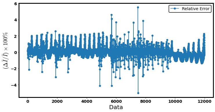
<AxesSubplot:xlabel='Data', ylabel='$(\\Delta\\bar{I}/\\bar{I})\\times 100\\%$'>
training_error_funct(df2, 'Ibar' , 'Ibar_model')
| train_Max_Error | d_max_training(%) | MAPE_taining(%) | |
|---|---|---|---|
| 0 | 1.495077 | 5.515113 | 0.359109 |
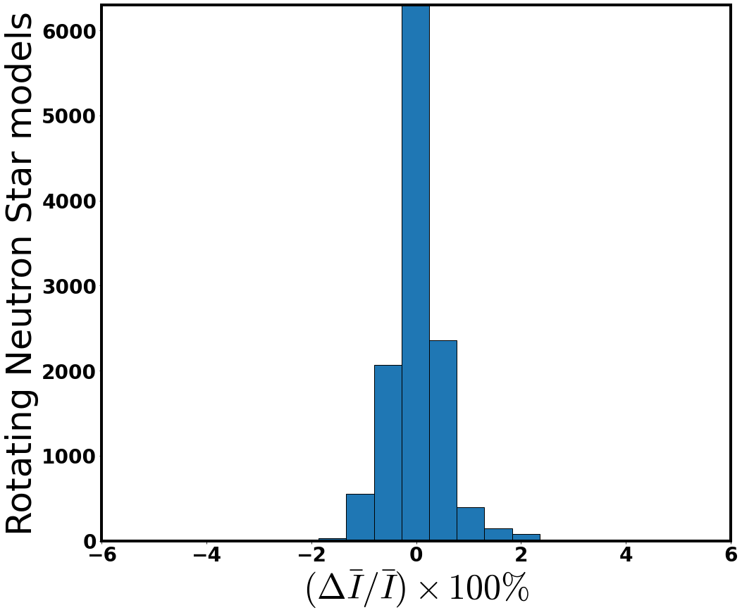
training_relative_error_hist(df2, 'Ibar', 'Ibar_model',
                             r'$(\Delta\bar{I}/\bar{I})\times 100\%$', r'Rotating Neutron Star models', n_bins=20,
                             x1_lim=-6, x2_lim=6)
Error distribution at space#
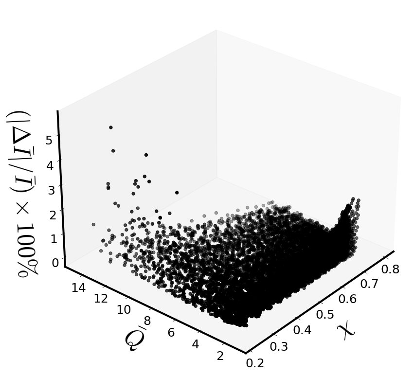
 relative_error_space_distribution(df2, 'x' , 'qbar' ,'Ibar','Ibar_model' ,
                                  '$\chi$',r'$\bar{Q}$', r'$(|\Delta\bar{I}|/\bar{I})\times 100\%$', view2=220)
Considerable relative deviations#
#variance_of_errors(df=df2,reference_deviation = 2,z = df2['Ibar'],z_model=df2['Ibar_model'])[['x','C','qbar','rel_error']]
variance_of_errors(df=df2,reference_deviation = 2,z = df2['Ibar'],z_model=df2['Ibar_model'])[['x','C','qbar']].min()
x       0.230938
C       0.100585
qbar    1.288669
dtype: float64
variance_of_errors(df=df2,reference_deviation = 2,z = df2['Ibar'],z_model=df2['Ibar_model'])[['x','C','qbar']].max()
x        0.721537
C        0.303458
qbar    13.200940
dtype: float64
Best Model’s optimizers-coefficients#
# model's intercept
d_00 = Regression_function(df2,x = 'x',y= 'qbar' ,z='Ibar', pol_degree=4, x_power = 'x',y_power='Qbar')[2]
# Other model's coefficients
d_nm = Regression_function(df2,x = 'x',y= 'qbar' ,z='Ibar', pol_degree=4, x_power = 'x',y_power='Qbar')[3]
# Coefficients stored to data frame
coef2=pd.DataFrame(d_nm,columns=["coef"])
powers2 = Regression_function(df2,x = 'x',y= 'qbar' ,z='Ibar',
                            pol_degree=4, x_power = 'x',y_power='Qbar')[5]
#powers2
def I_bar_funct(chi,qbar):
    results=0
    for i in range(0,len(coef2)):
        results +=(coef2["coef"][i]*chi**(powers2["x"][i])*qbar**(powers2["Qbar"][i]))
    return d_00+results
Model’s functional form \(\bar{I}=f(\chi,\bar{Q})\)#
I_bar_funct(chi_s,qbar_s).collect(chi_s)
\[\displaystyle 4.12814923032722 \chi^{4} + \chi^{3} \left(- 0.191023525347777 {\left(\bar{Q}\right)} - 5.90221583422805\right) + \chi^{2} \left(- 0.00988701228039328 {\left(\bar{Q}\right)}^{2} + 2.5042416840364 {\left(\bar{Q}\right)} + 0.270699315112401\right) + \chi \left(0.00323171728186578 {\left(\bar{Q}\right)}^{3} - 0.0642869194795781 {\left(\bar{Q}\right)}^{2} + 0.368224696809718 {\left(\bar{Q}\right)} - 1.06815685062771\right) - 0.000471467663097025 {\left(\bar{Q}\right)}^{4} + 0.0140174223624556 {\left(\bar{Q}\right)}^{3} - 0.113223649616265 {\left(\bar{Q}\right)}^{2} + 2.12361299011913 {\left(\bar{Q}\right)} + 2.07832395938375\]
Characteristic curves for different values of \(\chi\)#
Yagi and Yunes fitting formula for slowly rotating NSs#
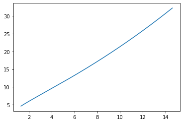
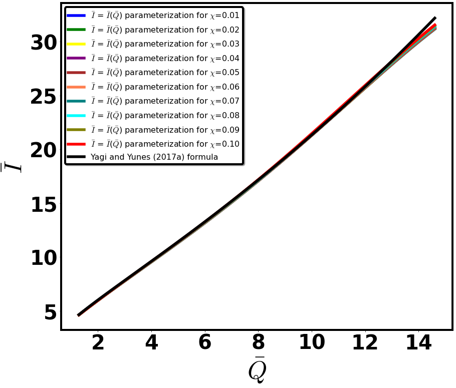
def YY_Ibar_Qbar(x):
    lny = 1.393 + 0.5471*np.log(x)+0.03028*(np.log(x))**2 + 0.01926*(np.log(x))**3+ 4.434*10**(-4)*(np.log(x))**4
    y = np.exp(lny)
    return y
chi_data = np.arange(0.01,0.11,0.01)
df2['q_values_test'] = np.linspace(df2['qbar'].min(), df2['qbar'].max() ,num = len(df2))
plt.plot(df2['q_values_test'],YY_Ibar_Qbar(df2['q_values_test']))
[<matplotlib.lines.Line2D at 0x7f4ba14eeaf0>]
I_bar_model_curve_fits(df2, x='q_values_test',y=chi_data, xlabel=r'$\bar{Q} $', ylabel=r"$\bar{I}$", fig_label=r"$\chi$")
Model curve fits compared to data#
df2_x_0_23=df2[(df2['x']>=0.228) & (df2['x']<=0.234)].copy()
df2_x_0_23.reset_index(drop=True, inplace=True)
#------------------------------------------------------------------
df2_x_0_3=df2[(df2['x']>=0.29) & (df2['x']<=0.31)].copy()
df2_x_0_3.reset_index(drop=True, inplace=True)
#----------------------------------------------------------------
df2_x_0_5=df2[(df2['x']>=0.495) & (df2['x']<=0.504)].copy()
df2_x_0_5.reset_index(drop=True, inplace=True)
#----------------------------------------------------------------
df2_x_0_7=df2[(df2['x']>=0.695) & (df2['x']<=0.704)].copy()
df2_x_0_7.reset_index(drop=True, inplace=True)
#----------------------------------------------------------------

df_chi_data = [df2_x_0_23,df2_x_0_3, df2_x_0_5, df2_x_0_7]

q_data = np.linspace(df2['qbar'].min(), df2['qbar'].max(),50)
I_data = np.linspace(df2['Ibar'].min(), df2['Ibar'].max(),50)
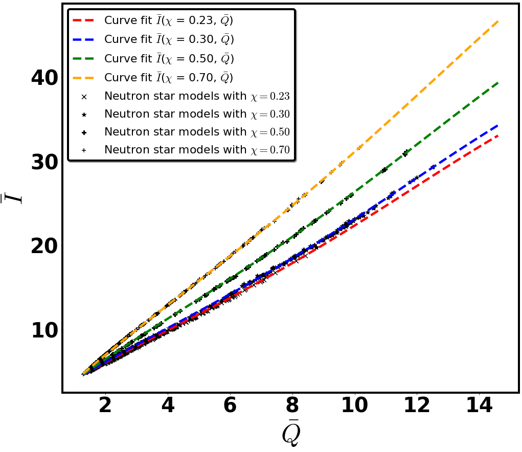
def Qbar_curve_fits_compared_to_chi_data(data_list, x,z, x_data, z_data, xlabel,zlabel):

    markers = ["x", "*", "P", "+"]
    chi = np.array([0.23,0.3,0.5,0.7])
    color2 = ["red","blue","green","orange"]

    #plt.figure(figsize=(16, 14))
    fig,ax = plt.subplots(figsize=(16, 14),)
    labels_text_size = 50
    font_size = 40
    scatter_size = 75

    plt.xticks(fontsize=font_size, fontweight="bold")
    plt.yticks(fontsize=font_size, fontweight="bold")
    plt.xlabel(xlabel,size=labels_text_size )
    plt.ylabel(zlabel,size=labels_text_size )

    for i in range(0,len(data_list)):
        plt.scatter((data_list[i][x]),(data_list[i][z]),color='black',s=scatter_size,
                    marker=markers[i] ,label = f"Neutron star models with $\chi={chi[i]:0.2f}$")

        plt.plot((x_data),(I_bar_funct(chi[i],x_data)),color=color2[i], lw = 4.5, ls = '--',
                    label = f"Curve fit {zlabel}($\chi$ = {chi[i]:0.2f}, {xlabel})")

    for axis in ['top','bottom','left','right']:
        ax.spines[axis].set_linewidth(4.0)

    leg = plt.legend(loc="best", prop={'size': 22}, shadow=True, fontsize="large", ncol = 1)
    leg.get_frame().set_linewidth(4.0)
    leg.get_frame().set_edgecolor('black')


    plt.grid(False)

    #plt.savefig('Ibar_chi_fixed_qbar.png',dpi=100,facecolor="w", bbox_inches='tight',transparent=True, pad_inches=0.2)

    plt.show()
Qbar_curve_fits_compared_to_chi_data(df_chi_data, 'qbar','Ibar', x_data=q_data,
                                     z_data=I_data , xlabel=r'$\bar{Q}$',zlabel=r'$\bar{I}$')
Fitting Surface compared to data#
x2 = mesh_grid_funct(df2,x_name = 'x', y_name = 'qbar')[0]
y2 = mesh_grid_funct(df2,x_name = 'x', y_name = 'qbar')[1]
Z_2 = I_bar_funct(x2,y2)
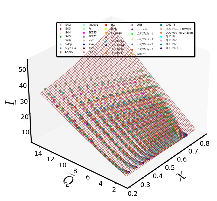
Surface_plot_funct_2(eos_data, 'x','q_tilde_GH','Ibar', xlabel='$\chi$',ylabel=r'$\bar{Q}$',zlabel=r'$\bar{I}$',
                     view2=220, n_col=5, border_axes=8, X=x2,Y=y2,Z=Z_2, l_w=1.5)
Investigation of the \(\bar{I}=\bar{I}(\sigma,\bar{Q})\) parameterization#
df3 = {'C':C,'sigma': sigma, 'M*f/c':M_x_f,'qbar': quadr, 'Ibar':I_bar}
df3=pd.DataFrame(data=df3, index=None, columns=None, dtype=None, copy=False)
df3.reset_index(drop=True, inplace=True)
#df3
Cross validation statistical metrics and results for different ‘pol degrees’ \(\kappa\)#
#cv_results = c_val_performace_results_for_k(df3,x='sigma',y='qbar',z='Ibar')
#cv_results
pd.read_csv(r"LOOCV_results/Ibar_sigma_Qbar_cv_scores.txt", sep=' ')
# best functional form form for pol_degree = 4
| MAE | Max_Error | MSE | d(%) | MAPE(%) | Explained_Variance | k | |
|---|---|---|---|---|---|---|---|
| 0 | 0.189678 | 2.645779 | 0.087088 | 10.964253 | 1.772847 | 1.0 | 2.0 |
| 1 | 0.127812 | 1.686365 | 0.049712 | 6.996384 | 1.008906 | 1.0 | 3.0 |
| 2 | 0.117109 | 1.608137 | 0.046497 | 6.661779 | 0.863887 | 1.0 | 4.0 |
| 3 | 0.116360 | 1.598041 | 0.046296 | 6.607161 | 0.852767 | 1.0 | 5.0 |
| 4 | 0.131275 | 1.820526 | 0.049596 | 7.544357 | 1.058312 | 1.0 | 6.0 |
| 5 | 0.115401 | 1.799478 | 0.044202 | 7.457133 | 0.861302 | 1.0 | 7.0 |
Linear Regression at training data#
df3['Ibar_model'] = Regression_function(df3,x = 'sigma',y= 'qbar' ,z='Ibar', pol_degree=4, x_power = 'sigma',y_power='Qbar')[0]
#df3['Ibar_model']
\(R^2\) - quality index#
Regression_function(df3,x = 'sigma',y= 'qbar' ,z='Ibar', pol_degree=4, x_power = 'sigma',y_power='Qbar')[1]
0.9987773278909703
Evaluation functions at training data#
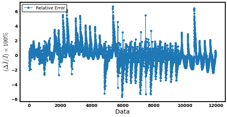
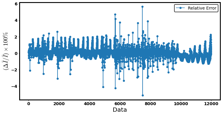
relative_training_error_plot(df3, 'Ibar' , 'Ibar_model', xlabel='Data', ylabel=r'$(\Delta\bar{I}/\bar{I})\times 100\%$')
<AxesSubplot:xlabel='Data', ylabel='$(\\Delta\\bar{I}/\\bar{I})\\times 100\\%$'>
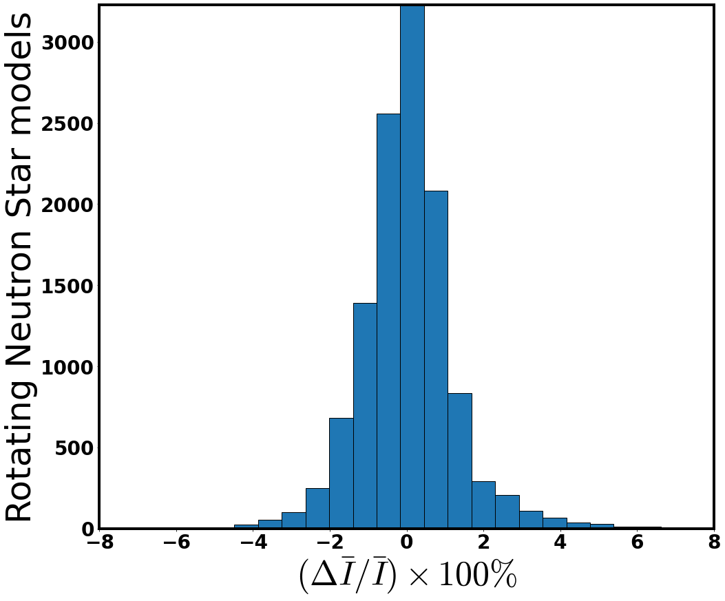
training_error_funct(df3, 'Ibar' , 'Ibar_model')
| train_Max_Error | d_max_training(%) | MAPE_taining(%) | |
|---|---|---|---|
| 0 | 1.600621 | 6.626827 | 0.862424 |
training_relative_error_hist(df3, 'Ibar', 'Ibar_model',
                             r'$(\Delta\bar{I}/\bar{I})\times 100\%$', r'Rotating Neutron Star models',n_bins=20,
                             x1_lim=-8., x2_lim=8)
Error distribution at space#
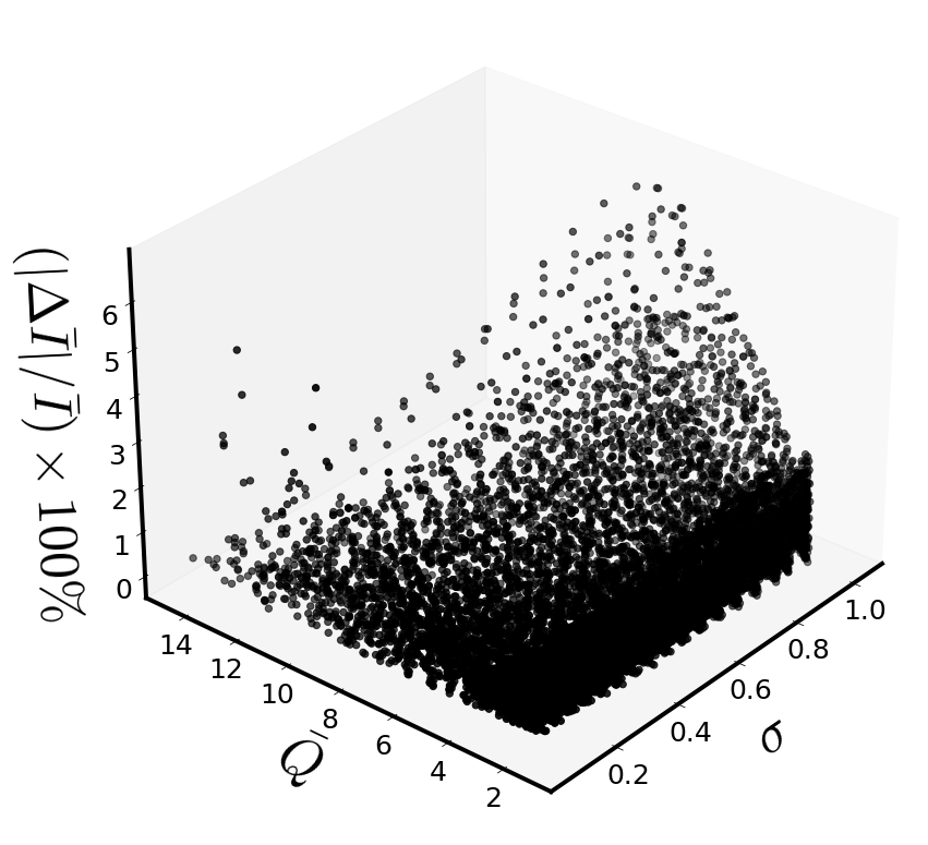
relative_error_space_distribution(df3, 'sigma' , 'qbar' ,'Ibar','Ibar_model' ,
                                  r'$\sigma$',r'${\bar{Q}}$', r'$(|\Delta\bar{I}|/\bar{I})\times 100\%$', view2=220)
Considerable relative deviations#
#variance_of_errors(df=df3,reference_deviation = 4,z = df3['Ibar'],z_model=df3['Ibar_model'])[['sigma','C','qbar','rel_error']]
variance_of_errors(df=df3,reference_deviation = 4,z = df3['Ibar'],z_model=df3['Ibar_model'])[['sigma','C','qbar']].min()
sigma    0.069236
C        0.085746
qbar     4.811075
dtype: float64
variance_of_errors(df=df3,reference_deviation = 4,z = df3['Ibar'],z_model=df3['Ibar_model'])[['sigma','C','qbar']].max()
sigma     1.032694
C         0.146504
qbar     12.528758
dtype: float64
Best Model’s optimizers-coefficients#
#Model's intercept
e_00 = Regression_function(df3,x = 'sigma',y= 'qbar' ,z='Ibar', pol_degree=4, x_power = 'sigma',y_power='Qbar')[2]
# Other model's coefficients
e_nm = Regression_function(df3,x = 'sigma',y= 'qbar' ,z='Ibar', pol_degree=4, x_power = 'sigma',y_power='Qbar')[3]
# results stored in data frame
coef3=pd.DataFrame(e_nm,columns=["coef"])
#coef3
#Regression_function(df3,x = 'sigma',y= 'qbar' ,z='Ibar', pol_degree=4, x_power = 'sigma',y_power='Qbar')[4]
powers3 = Regression_function(df3,x = 'sigma',y= 'qbar' ,z='Ibar', pol_degree=4,
                              x_power = 'sigma',y_power='Qbar')[5]
#powers3
def Ibar_sigma_Qbar(sigma,qbar):
    results=0
    for i in range(0,len(coef3)):
        results += (coef3["coef"][i]*sigma**(powers3["sigma"][i])*qbar**(powers3["Qbar"][i]))
    return e_00 + results
Regression Function#
Ibar_sigma_Qbar(sigma_s,qbar_s).collect(sigma_s)
\[\displaystyle 1.01625388262427 \sigma^{4} + \sigma^{3} \left(- 0.794692150355151 {\left(\bar{Q}\right)} - 1.00396747187348\right) + \sigma^{2} \left(- 0.0153327681904299 {\left(\bar{Q}\right)}^{2} + 0.31569363230144 {\left(\bar{Q}\right)} + 0.867628004467312\right) + \sigma \left(0.00813759299575639 {\left(\bar{Q}\right)}^{3} - 0.0911470112768361 {\left(\bar{Q}\right)}^{2} + 2.09378347244096 {\left(\bar{Q}\right)} - 2.75581919692545\right) - 0.000259078914026212 {\left(\bar{Q}\right)}^{4} + 0.00841524473738142 {\left(\bar{Q}\right)}^{3} - 0.0672539855778538 {\left(\bar{Q}\right)}^{2} + 1.99796863689949 {\left(\bar{Q}\right)} + 2.18837088409015\]
Indicative Curve fits#
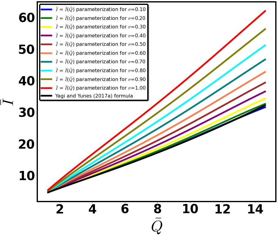
sigma_values = np.arange(0.1,1.1,0.1)
df3['q_values_test'] = np.linspace(df3['qbar'].min(), df2['qbar'].max() ,num = len(df2))
I_bar_model_curve_fits(df3, x='q_values_test',y=sigma_values, xlabel=r'$\bar{Q}$', ylabel=r"$\bar{I}$", fig_label=r"$\sigma$")
Fitting Surface compared to data#
x3 = mesh_grid_funct(df3,x_name = 'sigma', y_name = 'qbar')[0]
y3 = mesh_grid_funct(df3,x_name = 'sigma', y_name = 'qbar')[1]
Z_3 = Ibar_sigma_Qbar(x3,y3)
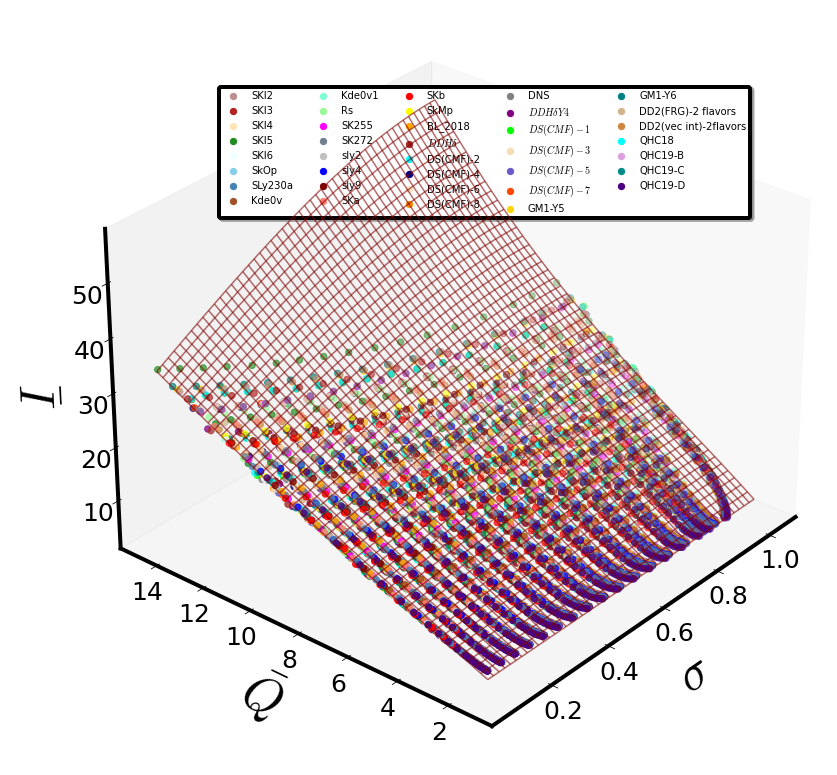
Surface_plot_funct_2(eos_data, 'sigma','q_tilde_GH','Ibar', xlabel=r'$\sigma$',ylabel=r'${\bar{Q}}$',zlabel=r'${\bar{I}}$',
                     view2=220, n_col=5, border_axes=8, X=x3,Y=y3,Z=Z_3, l_w=1.5)
Investigation of the \(\bar{I}=\bar{I}(\mathcal{E},\bar{Q})\) parameterization, where \(\mathcal{E}= T/|W|\)#
df4 = {'C': C,'T/W': T_over_W, 'qbar': quadr, 'Ibar':I_bar}
df4=pd.DataFrame(data=df4, index=None, columns=None, dtype=None, copy=False)
df4.reset_index(drop=True, inplace=True)
#df4
Cross validation statistical metrics and results for different ‘pol degrees’ \(\kappa\)#
#cv_results = c_val_performace_results_for_k(df4,x='T/W',y='qbar',z='Ibar')
#cv_results
pd.read_csv(r"LOOCV_results/Ibar_T_W_Qbar_cv_scores.txt", sep=' ')
# best functional form form for pol_degree = 4
| MAE | Max_Error | MSE | d(%) | MAPE(%) | Explained_Variance | k | |
|---|---|---|---|---|---|---|---|
| 0 | 0.073430 | 1.730219 | 0.011180 | 6.382517 | 0.729715 | 1.0 | 2.0 |
| 1 | 0.042795 | 1.556876 | 0.004683 | 5.743079 | 0.469486 | 1.0 | 3.0 |
| 2 | 0.032337 | 1.547112 | 0.003586 | 5.707060 | 0.334542 | 1.0 | 4.0 |
| 3 | 0.028758 | 1.531283 | 0.003263 | 5.648669 | 0.286031 | 1.0 | 5.0 |
| 4 | 0.027257 | 1.621370 | 0.003140 | 5.980986 | 0.267788 | 1.0 | 6.0 |
| 5 | 0.026905 | 1.616781 | 0.003103 | 5.964060 | 0.263152 | 1.0 | 7.0 |
Linear Regression at training data#
df4['Ibar_model'] = Regression_function(df4,x = 'T/W',y= 'qbar' ,z='Ibar', pol_degree=4, x_power = 'T/W',y_power='Qbar')[0]
#df4['Ibar_model']
\(R^2\) - quality index#
Regression_function(df4,x = 'T/W',y= 'qbar' ,z='Ibar', pol_degree=4, x_power = 'T/W',y_power='Qbar')[1]
0.9999061377438476
Evaluation functions at training data#
relative_training_error_plot(df4, 'Ibar' , 'Ibar_model', xlabel='Data', ylabel=r'$(\Delta\bar{I}/\bar{I})\times 100\%$')
<AxesSubplot:xlabel='Data', ylabel='$(\\Delta\\bar{I}/\\bar{I})\\times 100\\%$'>
training_error_funct(df4, 'Ibar' , 'Ibar_model')
| train_Max_Error | d_max_training(%) | MAPE_taining(%) | |
|---|---|---|---|
| 0 | 1.527418 | 5.634414 | 0.334046 |
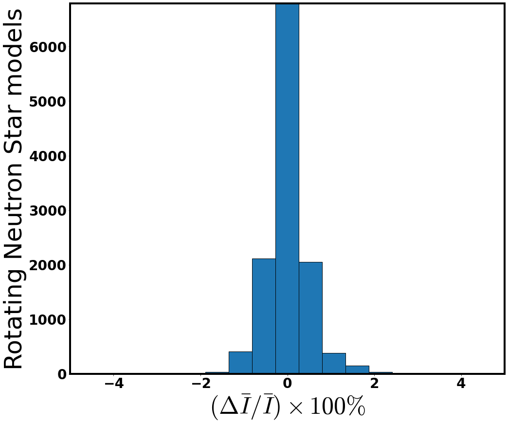
training_relative_error_hist(df4, 'Ibar', 'Ibar_model',
                             r'$(\Delta\bar{I}/\bar{I})\times 100\%$', r'Rotating Neutron Star models',n_bins=20,
                             x1_lim=-5, x2_lim=5)
Error distribution at space#
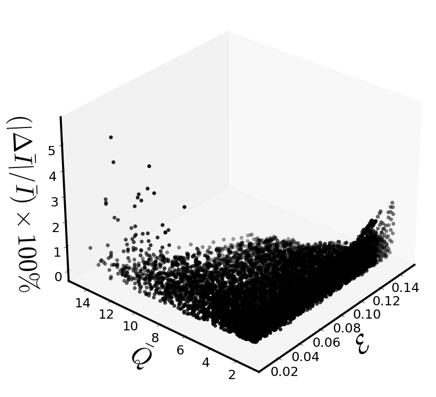
relative_error_space_distribution(df4, 'T/W' , 'qbar' ,'Ibar','Ibar_model' ,
                                  r'$\mathcal{E}$',r'$\bar{Q}$', r'$(|\Delta\bar{I}|/\bar{I})\times 100\%$',
                                  view2=220)
Considerable relative deviations#
#variance_of_errors(df=df4,reference_deviation = 2,z = df4['Ibar'],z_model=df4['Ibar_model'])[['T/W','C','Ibar','rel_error']]
len(variance_of_errors(df=df4,reference_deviation = 2,z = df4['Ibar'],z_model=df4['Ibar_model'])[['T/W','C','Ibar','rel_error']])
50
variance_of_errors(df=df4,reference_deviation = 2,z = df4['Ibar'],z_model=df4['Ibar_model'])[['T/W','C','Ibar']].min()
T/W     0.012328
C       0.100585
Ibar    4.671020
dtype: float64
variance_of_errors(df=df4,reference_deviation = 2,z = df4['Ibar'],z_model=df4['Ibar_model'])[['T/W','C','Ibar']].max()
T/W      0.143318
C        0.300582
Ibar    31.340543
dtype: float64
Best Model’s optimizers-coefficients#
#model's intercept
f_00 = Regression_function(df4,x = 'T/W',y= 'qbar' ,z='Ibar', pol_degree=4, x_power = 'T/W',y_power='Qbar')[2]
#Other model's coefficient
f_nm = Regression_function(df4,x = 'T/W',y= 'qbar' ,z='Ibar', pol_degree=4, x_power = 'T/W',y_power='Qbar')[3]
#Results stored to data frame
coef4=pd.DataFrame(f_nm,columns=["coef"])
#Regression_function(df4,x = 'T/W',y= 'qbar' ,z='Ibar', pol_degree=4, x_power = 'T/W',y_power='Qbar')[4]
powers4 = Regression_function(df4,x = 'T/W',y= 'qbar' ,z='Ibar',
                              pol_degree=4, x_power = 'T/W',y_power='Qbar')[5]
#powers4
def Ibar_tw_qbar(TW, qbar):
    results=0
    for i in range(0,len(coef4)):
        results += (coef4["coef"][i]*TW**(powers4["T/W"][i])*qbar**(powers4["Qbar"][i]))
    return f_00+results
Regression function#
Ibar_tw_qbar(TW_s, qbar_s).collect(TW_s)
\[\displaystyle 1850.99483675157 \mathcal{E}^{4} + \mathcal{E}^{3} \left(73.0543232250824 {\left(\bar{Q}\right)} - 531.206777460634\right) + \mathcal{E}^{2} \left(3.050817416506 {\left(\bar{Q}\right)}^{2} - 15.7943004600174 {\left(\bar{Q}\right)} + 42.9442258499973\right) + \mathcal{E} \left(0.017713904016752 {\left(\bar{Q}\right)}^{3} - 0.0500904059425615 {\left(\bar{Q}\right)}^{2} + 9.34741625474308 {\left(\bar{Q}\right)} - 11.3443000684699\right) - 0.000402647010270485 {\left(\bar{Q}\right)}^{4} + 0.0126259849746673 {\left(\bar{Q}\right)}^{3} - 0.105637908493565 {\left(\bar{Q}\right)}^{2} + 2.11773355691406 {\left(\bar{Q}\right)} + 2.04285931818562\]
Fitting Surface compared to data#
x4 = mesh_grid_funct(df4,x_name = 'T/W', y_name = 'qbar')[0]
y4 = mesh_grid_funct(df4,x_name = 'T/W', y_name = 'qbar')[1]
Z_4 = Ibar_tw_qbar(x4,y4)
Surface_plot_funct_2(eos_data, 'T/W','q_tilde_GH','Ibar', xlabel=r'$\mathcal{E}$',ylabel=r'$\bar{Q}$',zlabel=r'$\bar{I}$',
                     view2=220, n_col=5, border_axes=1, X=x4,Y=y4,Z=Z_4, l_w=1.5)
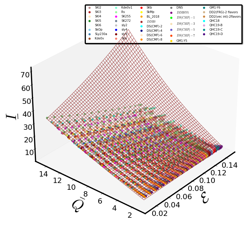
Investigation of the correlation \(\bar{I} = \bar{I}(R(km)\times \frac{f(Hz)}{c},\bar{Q})\)#
df4_b = {'C':C,'x': x_spin, 'sigma':sigma, "f(kHz)":f_kHz,'M*f/c':M_x_f, "R*f/c": R_x_f,'qbar': quadr,
         'M*f/x':M_f_over_x,'Ibar':I_bar,'S3bar':S3_bar}
df4_b = pd.DataFrame(data=df4_b, index=None, columns=None, dtype=None, copy=False)
df4_b.reset_index(drop=True, inplace=True)
Cross validation statistical metrics and results for different ‘pol degrees’ \(\kappa\)#
#cv_results = c_val_performace_results_for_k(df4_b,x='R*f/c',y='qbar',z='Ibar')
#cv_results
pd.read_csv(r"LOOCV_results/Inar_Rf_barQ_cv_scores.txt", sep=' ')
# best functional form form for pol_degree = 2
| MAE | Max_Error | MSE | d(%) | MAPE(%) | Explained_Variance | k | |
|---|---|---|---|---|---|---|---|
| 0 | 0.151944 | 1.868130 | 0.065331 | 7.308533 | 1.275055 | 1.0 | 2.0 |
| 1 | 0.120213 | 1.978032 | 0.048932 | 8.197073 | 0.907791 | 1.0 | 3.0 |
| 2 | 0.112795 | 1.874424 | 0.042097 | 7.767715 | 0.875946 | 1.0 | 4.0 |
| 3 | 0.105622 | 1.751490 | 0.039117 | 7.258272 | 0.784305 | 1.0 | 5.0 |
| 4 | 0.104532 | 1.715143 | 0.038781 | 7.107645 | 0.777119 | 1.0 | 6.0 |
| 5 | 0.111774 | 1.815012 | 0.040360 | 7.236214 | 0.876385 | 1.0 | 7.0 |
Linear Regression at training data#
df4_b['Ibar_model'] = Regression_function(df4_b,x = 'R*f/c',y= 'qbar' ,z='Ibar', pol_degree=2, x_power = 'R*f/c',y_power='Qbar')[0]
#df['Ibar_model']
\(R^2\) - quality index#
Regression_function(df4_b,x = 'R*f/c',y= 'qbar' ,z='Ibar', pol_degree=2, x_power = 'R*f/c',y_power='Qbar')[1]
0.998272657227808
Evaluation functions at training data#
relative_training_error_plot(df4_b, 'Ibar' , 'Ibar_model', xlabel='Data', ylabel=r'$(\Delta\bar{I}/\bar{I})\times 100\%$')
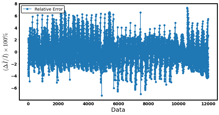
<AxesSubplot:xlabel='Data', ylabel='$(\\Delta\\bar{I}/\\bar{I})\\times 100\\%$'>
training_error_funct(df4_b, 'Ibar' , 'Ibar_model')
| train_Max_Error | d_max_training(%) | MAPE_taining(%) | |
|---|---|---|---|
| 0 | 1.865616 | 7.300936 | 1.274266 |
training_relative_error_hist(df4_b, 'Ibar', 'Ibar_model',
                             r'$(\Delta\bar{I}/\bar{I})\times 100\%$', r'Rotating Neutron Star models',n_bins = 20,
                             x1_lim=-10, x2_lim=10)
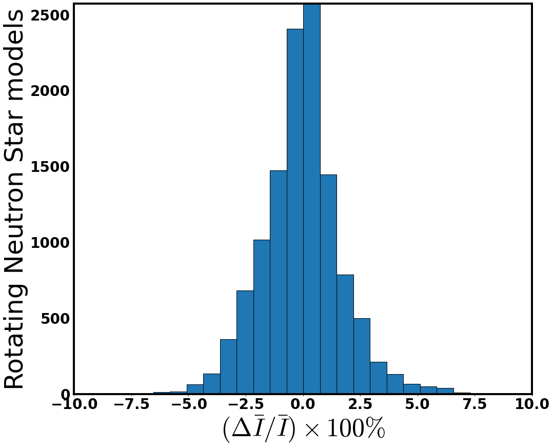
Error distribution at space#
relative_error_space_distribution(df4_b, 'R*f/c' , 'qbar' ,'Ibar','Ibar_model' ,
                                  r'$ R_{eq}\times \tilde{f}$',r'$\bar{Q}$', r'$(|\Delta\bar{I}|/\bar{I})\times 100\%$',
                                  view2=220)
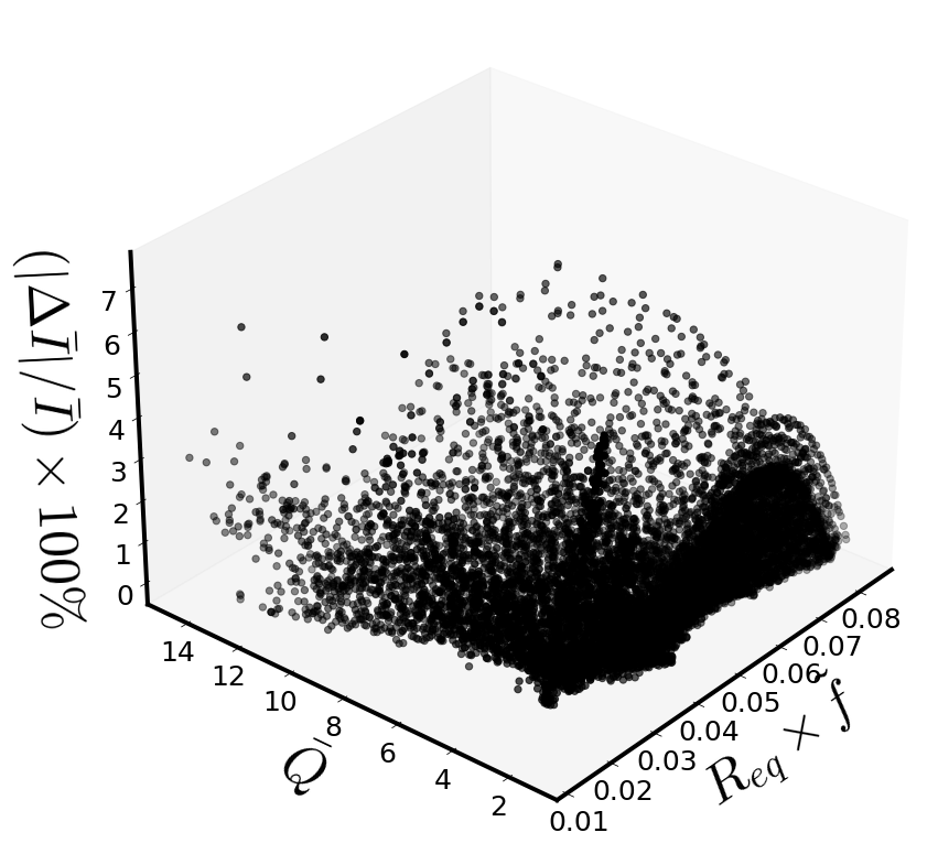
Variance of errors#
#variance_of_errors(df=df4_b,reference_deviation = 5,z = df4_b['Ibar'],z_model=df4_b['Ibar_model'])[['R*f/c','x','C','qbar']]
variance_of_errors(df=df4_b,reference_deviation = 5,z = df4_b['Ibar'],z_model=df4_b['Ibar_model'])[['R*f/c','x','C','qbar']].min()
R*f/c    0.013734
x        0.237689
C        0.090535
qbar     1.507171
dtype: float64
variance_of_errors(df=df4_b,reference_deviation = 5,z = df4_b['Ibar'],z_model=df4_b['Ibar_model'])[['R*f/c','x','C','qbar']].max()
R*f/c     0.064207
x         0.788718
C         0.310997
qbar     12.528758
dtype: float64
#variance_of_errors(df=df4_b, reference_deviation=5,z=df4_b['Ibar'],
#                   z_model=df4_b['Ibar_model'])[['qbar','R*f/c','C','x','rel_error']]
variance_of_errors(df=df4_b, reference_deviation=5,z=df4_b['Ibar'],
                   z_model=df4_b['Ibar_model'])[['x','C']].min()
x    0.237689
C    0.090535
dtype: float64
variance_of_errors(df=df4_b, reference_deviation=5,z=df4_b['Ibar'],
                   z_model=df4_b['Ibar_model'])[['x','C']].max()
x    0.788718
C    0.310997
dtype: float64
Best Model’s optimizers-coefficients#
# model's intercept
A_00 = Regression_function(df4_b,x = 'R*f/c',y= 'qbar' ,z='Ibar', pol_degree=2, x_power = 'R*f/c',y_power='Qbar')[2]
# Other model's coefficients
A_nm = Regression_function(df4_b,x = 'R*f/c',y= 'qbar' ,z='Ibar', pol_degree=2, x_power = 'R*f/c',y_power='Qbar')[3]
#Results stored in data frame
coef4_b=pd.DataFrame(A_nm,columns=["coef"])
#coef4b
#Regression_function(df4_b,x = 'R*f/c',y= 'qbar' ,z='Ibar', pol_degree=2, x_power = 'R*f/c',y_power='Qbar')[4]
powers4_b = Regression_function(df4_b,x = 'R*f/c',y= 'qbar' ,z='Ibar', pol_degree=2,
                                x_power = 'R*f/c',y_power='Qbar')[5]
#powers_4b
def I_bar_Rf_qbar(x,y):
    results=0
    for i in range(0,len(powers4_b)):
        results+=(coef4_b["coef"][i]*x**(powers4_b["R*f/c"][i])*y**(powers4_b["Qbar"][i]))

    return A_00 + results
Fitting Surface compared to data#
x4_b = mesh_grid_funct(df4_b,x_name = 'R*f/c', y_name = 'qbar')[0]
y4_b = mesh_grid_funct(df4_b,x_name = 'R*f/c', y_name = 'qbar')[1]
Z4_b = I_bar_Rf_qbar(x4_b, y4_b)
Surface_plot_funct_2(eos_data, 'R*f/c','q_tilde_GH','Ibar', xlabel=r'$ R_{eq}\times \tilde{f}$',ylabel=r'$\bar{Q}$',zlabel=r'$\bar{I}$',
                     view2=220, n_col=5, border_axes=1, X=x4_b,Y=y4_b,Z=Z4_b, l_w=1.5)
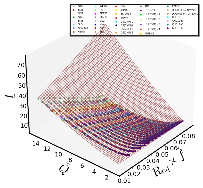
Investigation of the \(\bar{S_3}= \bar{S_3}(\chi,\bar{I})\) parameterization#
df5 = {'C':C,'x': x_spin,'sigma':sigma,'M*f/c':M_x_f,'R*f/c':R_x_f,'Ibar': I_bar, 'S3bar':S3_bar}
df5=pd.DataFrame(data=df5, index=None, columns=None, dtype=None, copy=False)
df5.reset_index(drop=True, inplace=True)
#df5
————– comment ————————#
Cross validation process for the \(\bar{S_3}= \bar{S_3}(\sigma,C)\) parameterization#
#cv_results = c_val_performace_results_for_k(df5,x='sigma',y='C',z='S3bar')
#cv_results
pd.read_csv(r"LOOCV_results/S3bar_C_sigma_cv_scores.txt", sep=' ')
| MAE | Max_Error | MSE | d(%) | MAPE(%) | Explained_Variance | k | |
|---|---|---|---|---|---|---|---|
| 0 | 0.522260 | 5.725634 | 0.473610 | 143.272606 | 10.061061 | 1.0 | 2.0 |
| 1 | 0.212453 | 2.479743 | 0.092392 | 64.275418 | 3.577843 | 1.0 | 3.0 |
| 2 | 0.152195 | 2.030365 | 0.054404 | 23.278895 | 1.986440 | 1.0 | 4.0 |
| 3 | 0.146739 | 1.974519 | 0.050631 | 11.531595 | 1.853457 | 1.0 | 5.0 |
| 4 | 0.154921 | 2.136282 | 0.053076 | 23.333604 | 2.128292 | 1.0 | 6.0 |
| 5 | 0.143050 | 2.016909 | 0.049129 | 10.039799 | 1.762590 | 1.0 | 7.0 |
Cross validation process for the \(\bar{S_3}= \bar{S_3}(\chi,C)\) parameterization#
#cv_results = c_val_performace_results_for_k(df5,x='x',y='C',z='S3bar')
#cv_results
pd.read_csv(r"LOOCV_results/S3bar_C_chi_cv_scores.txt", sep=' ')
| MAE | Max_Error | MSE | d(%) | MAPE(%) | Explained_Variance | k | |
|---|---|---|---|---|---|---|---|
| 0 | 0.602228 | 5.382748 | 0.702683 | 134.167646 | 10.788240 | 1.0 | 2.0 |
| 1 | 0.362701 | 3.924850 | 0.325355 | 65.492624 | 5.192739 | 1.0 | 3.0 |
| 2 | 0.320600 | 4.168888 | 0.280657 | 25.361548 | 4.030828 | 1.0 | 4.0 |
| 3 | 0.310031 | 4.058758 | 0.268279 | 24.472312 | 3.773624 | 1.0 | 5.0 |
| 4 | 0.310295 | 3.928865 | 0.267235 | 24.160710 | 3.813946 | 1.0 | 6.0 |
| 5 | 0.304828 | 3.630850 | 0.261964 | 23.268634 | 3.692353 | 1.0 | 7.0 |
—————————————————-#
Cross validation process for the \(\bar{S_3}= \bar{S_3}(\chi,\bar{I})\) parameterization#
#cv_results = c_val_performace_results_for_k(df5,x='x',y='Ibar',z='S3bar')
#cv_results
pd.read_csv(r"LOOCV_results/S3bar_chi_Ibar_cv_scores.txt", sep=' ')
# best functional form form for pol_degree = 4
| MAE | Max_Error | MSE | d(%) | MAPE(%) | Explained_Variance | k | |
|---|---|---|---|---|---|---|---|
| 0 | 0.112829 | 2.306753 | 0.026194 | 16.367661 | 2.073974 | 1.0 | 2.0 |
| 1 | 0.089083 | 1.920698 | 0.017358 | 9.758474 | 1.441720 | 1.0 | 3.0 |
| 2 | 0.084758 | 1.846365 | 0.016317 | 9.380814 | 1.303575 | 1.0 | 4.0 |
| 3 | 0.084193 | 1.837755 | 0.016259 | 9.337065 | 1.279078 | 1.0 | 5.0 |
| 4 | 0.083589 | 1.882897 | 0.016131 | 9.566420 | 1.270835 | 1.0 | 6.0 |
| 5 | 0.083766 | 1.915318 | 0.016132 | 9.731142 | 1.275273 | 1.0 | 7.0 |
Linear Regression at training data#
df5['S3bar_model'] = Regression_function(df5,x = 'x',y= 'Ibar' ,z='S3bar', pol_degree=4, x_power = 'x',y_power='Ibar')[0]
#df5['S3bar_model']
\(R^2\) - quality index#
Regression_function(df5,x = 'x',y= 'Ibar' ,z='S3bar', pol_degree=4, x_power = 'x',y_power='Ibar')[1]
0.9994789941953126
Evaluation functions at training data#
relative_training_error_plot(df5, 'S3bar' , 'S3bar_model', xlabel='Data', ylabel=r'$(\Delta\bar{S_3}/\bar{S_3})\times 100\%$')
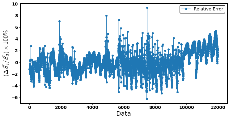
<AxesSubplot:xlabel='Data', ylabel='$(\\Delta\\bar{S_3}/\\bar{S_3})\\times 100\\%$'>
training_error_funct(df5, 'S3bar' , 'S3bar_model')
| train_Max_Error | d_max_training(%) | MAPE_taining(%) | |
|---|---|---|---|
| 0 | 1.836074 | 9.328529 | 1.30208 |
training_relative_error_hist(df5, 'S3bar', 'S3bar_model',
                             r'$(\Delta\bar{S_3}/\bar{S_3})\times 100\%$', r'Rotating Neutron Star models',n_bins=20,
                             x1_lim=-10, x2_lim=10)
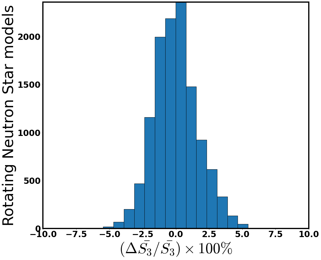
Error distribution at space#
relative_error_space_distribution(df5, 'x' , 'Ibar' ,'S3bar','S3bar_model' ,
                                  r'$\chi$',r'$\bar{I}$', r'$(|\Delta\bar{S}_3|/\bar{S}_3)\times 100\%$', view2=220)
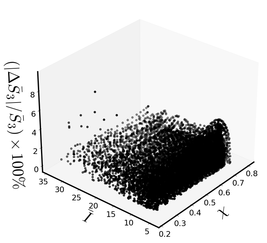
Considerable relative deviations#
#variance_of_errors(df=df5,reference_deviation = 5,z = df5['S3bar'],z_model=df5['S3bar_model'])[['x','C','Ibar']]
len(variance_of_errors(df=df5,reference_deviation = 5,z = df5['S3bar'],z_model=df5['S3bar_model'])[['x','C','Ibar']])
30
variance_of_errors(df=df5,reference_deviation = 5,z = df5['S3bar'],z_model=df5['S3bar_model'])[['x','C','Ibar']].min()
x       0.230379
C       0.107552
Ibar    5.369889
dtype: float64
variance_of_errors(df=df5,reference_deviation = 5,z = df5['S3bar'],z_model=df5['S3bar_model'])[['x','C','Ibar']].max()
x        0.666949
C        0.289819
Ibar    27.108734
dtype: float64
df5['C'].min()
0.08495475889382308
df5['x'].max()
0.7987388582866619
#df5['rel_error'] = 100*abs(df5['S3bar_model']-df5['S3bar'])/df5['S3bar']
#len(df5[df5['rel_error']>5])
#len(df5)
Best Model’s optimizers-coefficients#
#model's intercept
g_00 = Regression_function(df5,x = 'x',y= 'Ibar' ,z='S3bar', pol_degree=4, x_power = 'x',y_power='Ibar')[2]
#other model's coefficients
g_nm = Regression_function(df5,x = 'x',y= 'Ibar' ,z='S3bar', pol_degree=4, x_power = 'x',y_power='Ibar')[3]
#results stored in data frame
coef5=pd.DataFrame(g_nm,columns=["coef"])
#Regression_function(df5,x = 'x',y= 'Ibar' ,z='S3bar', pol_degree=4, x_power = 'x',y_power='Ibar')[4]
powers5 = Regression_function(df5,x = 'x',y= 'Ibar' ,z='S3bar', pol_degree=4, x_power = 'x',y_power='Ibar')[5]
#powers5
def S3_bar_x_Ibar(x,Ibar):
    results=0
    for i in range(0,len(powers5)):
        results+=(coef5["coef"][i]*x**(powers5["x"][i])*Ibar**(powers5["Ibar"][i]))

    return g_00 + results
Regression Function#
S3_bar_x_Ibar(chi_s,Ibar_s).collect(chi_s)
\[\displaystyle 1.46655568222798 \cdot 10^{-5} \bar{I}^{4} - 0.00117551458045689 \bar{I}^{3} + 0.0215999758403628 \bar{I}^{2} + 1.13258618353319 \bar{I} - 26.9132677137361 \chi^{4} + \chi^{3} \left(0.705537773391409 \bar{I} + 46.5772721491666\right) + \chi^{2} \left(- 0.00623582872477128 \bar{I}^{2} - 1.03818031162332 \bar{I} - 28.0868835154615\right) + \chi \left(1.6073925299509 \cdot 10^{-5} \bar{I}^{3} + 0.0173940691252201 \bar{I}^{2} - 0.571188445158182 \bar{I} + 11.6197481179223\right) - 4.93837426537477\]
Fitting Surface compared to data#
x5 = mesh_grid_funct(df5,x_name = 'x', y_name = 'Ibar')[0]
y5 = mesh_grid_funct(df5,x_name = 'x', y_name = 'Ibar')[1]

Z_5 = S3_bar_x_Ibar(x5,y5)
Surface_plot_funct_2(eos_data, 'x','Ibar','S3_bar_GH', xlabel=r'$\chi$',ylabel=r'$\bar{I}$',zlabel=r'$\bar{S}_3$',
                     view2=220, n_col=5, border_axes=8, X=x5,Y=y5,Z=Z_5, l_w=1.5)
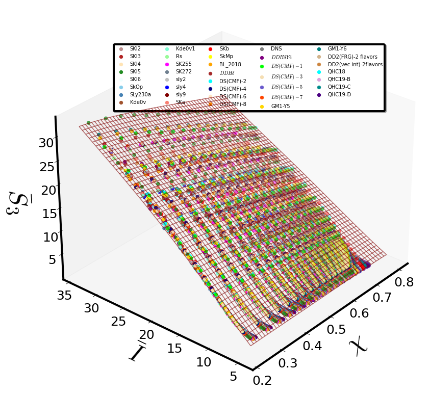
Investigation of the \(\bar{S}_3=f(\ln (\bar{Q}))\) parameterization#
df6 = {'C':C,'x':x_spin,'ln(qbar)': ln_Qbar, 'S3bar': S3_bar}
df6=pd.DataFrame(data=df6, index=None, columns=None, dtype=None, copy=False)
df6.reset_index(drop=True, inplace=True)
#df6
Cross validation statistical metrics and results for different ‘pol degrees’ \(\kappa\)#
#cv_results =c_val_performace_results_for_k_2(df6,x='ln(qbar)',z='S3bar')
#cv_results
pd.read_csv(r"LOOCV_results/S3bar_lnQbar_cv_scores.txt", sep=' ')
#best functional form form for pol_degree = 4
| MAE | Max_Error | MSE | d(%) | MAPE(%) | Explained_Variance | k | |
|---|---|---|---|---|---|---|---|
| 0 | 0.240152 | 2.842344 | 0.098319 | 45.553068 | 4.805720 | 1.0 | 2.0 |
| 1 | 0.094206 | 0.911921 | 0.017611 | 6.453714 | 1.437610 | 1.0 | 3.0 |
| 2 | 0.090383 | 0.893238 | 0.016711 | 4.846528 | 1.308325 | 1.0 | 4.0 |
| 3 | 0.090417 | 0.888842 | 0.016709 | 4.921987 | 1.311097 | 1.0 | 5.0 |
| 4 | 0.090362 | 0.886009 | 0.016710 | 4.912718 | 1.308350 | 1.0 | 6.0 |
| 5 | 0.090374 | 0.885954 | 0.016714 | 4.909781 | 1.308643 | 1.0 | 7.0 |
Linear Regression at training data#
df6['S3bar_model'] = Regression_function_2(df6,x = 'ln(qbar)' ,z='S3bar', pol_degree=4, x_power = 'lnQbar')[0]
#df6['S3bar_model']
\(R^2\) - quality index#
Regression_function_2(df6,x = 'ln(qbar)' ,z='S3bar', pol_degree=4, x_power = 'lnQbar')[1]
0.999463029026018
Evaluation functions at training data#
relative_training_error_plot(df6, 'S3bar' , 'S3bar_model', xlabel=r'$Data$', ylabel=r'$(\Delta\bar{S}_3/\bar{S}_3)\times 100\%$')
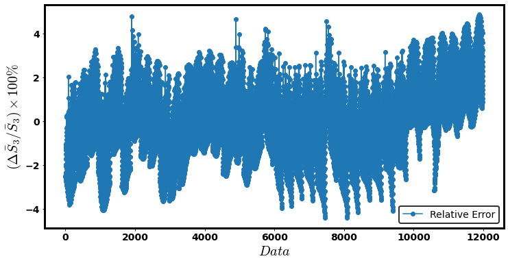
<AxesSubplot:xlabel='$Data$', ylabel='$(\\Delta\\bar{S}_3/\\bar{S}_3)\\times 100\\%$'>
training_error_funct(df6, 'S3bar' , 'S3bar_model')
| train_Max_Error | d_max_training(%) | MAPE_taining(%) | |
|---|---|---|---|
| 0 | 0.892562 | 4.845258 | 1.307847 |
training_relative_error_hist(df6, 'S3bar', 'S3bar_model',
                             r'$(\Delta\bar{S}_3/\bar{S}_3)\times 100\%$', r'Rotating Neutron Star models',n_bins=20,
                             x1_lim=-10, x2_lim=10)
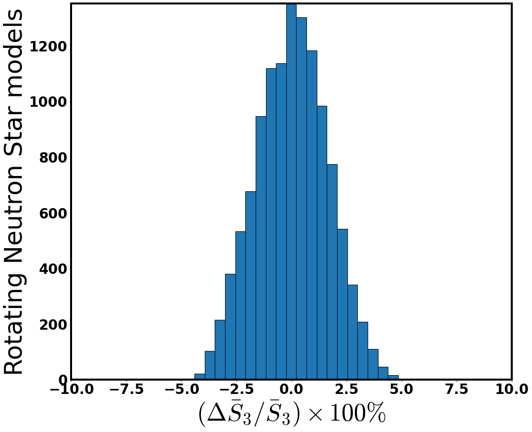
Best Model’s optimizers-coefficients#
model’s intercept#
# model's intercept
h_00 = Regression_function_2(df6,x = 'ln(qbar)' ,z='S3bar', pol_degree=4, x_power = 'lnQbar')[2]
# Other regression coefficients
h_nm = Regression_function_2(df6,x = 'ln(qbar)' ,z='S3bar', pol_degree=4, x_power = 'lnQbar')[3]
#Results stored in data frame
coef6=pd.DataFrame(h_nm,columns=["coef"])
#coef6
powers6 = Regression_function_2(df6,x = 'ln(qbar)' ,z='S3bar', pol_degree=4, x_power = 'lnQbar')[5]
#powers6
def S3bar_Curv(lnQbar):
    results = 0
    for i in range(0,len(coef6)):
        results +=(coef6["coef"][i]*lnQbar**(powers6["lnQbar"][i]))
    return results + h_00
Regression Function#
S3bar_Curv(lnQbar_s)
\[\displaystyle 0.270181812803186 \left(\ln{\bar{Q}}\right)^{4} + 0.03711000724575 \left(\ln{\bar{Q}}\right)^{3} + 1.36247243961029 \left(\ln{\bar{Q}}\right)^{2} + 2.24810590132046 \left(\ln{\bar{Q}}\right) + 1.02012141197205\]
lnq_data = np.linspace(df6['ln(qbar)'].min(), df6['ln(qbar)'].max(),100)
Z_6 = S3bar_Curv(lnq_data)
Error distribution#
relative_error_2D_distribution(df6, x='ln(qbar)', z='S3bar', z_trial='S3bar_model',
                               xlabel=r'$\ln\bar{Q}$', zlabel=r'$\left(|\Delta \bar{S}_3|/\bar{S}_3\right)\times 100\%$')
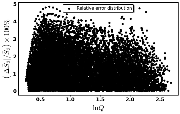
relative_error_2D_distribution_colored(eos_data, x='ln(qbar)',z='S3_bar_GH',
                                     xlabel=r'$\ln\bar{Q}$',
                                     zlabel=r'$\left(|\Delta \bar{S}_3|/\bar{S}_3\right)\times 100\%$',
                                     z_min =0,z_max=7, n_col=5)
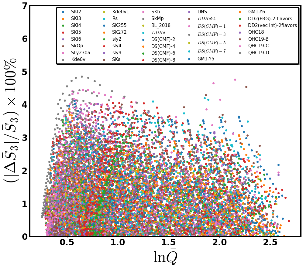
Considerable relative deviations ?#
#variance_of_errors(df=df6,reference_deviation = 4,z = df6['S3bar'],z_model=df6['S3bar_model'])[['x','C']]
variance_of_errors(df=df6,reference_deviation = 3,z = df6['S3bar'],z_model=df6['S3bar_model'])[['x','C']].min()
x    0.229089
C    0.085746
dtype: float64
variance_of_errors(df=df6,reference_deviation = 3,z = df6['S3bar'],z_model=df6['S3bar_model'])[['x','C']].max()
x    0.744331
C    0.311708
dtype: float64
Curve fit compared to data#
fitting_curve(eos_data, x='ln(qbar)',z='S3_bar_GH', xlabel=r'$\ln\bar{Q}$', zlabel=r'$\bar{S}_3$',
              X=lnq_data,Z=Z_6, l_w=8, n_col=4)
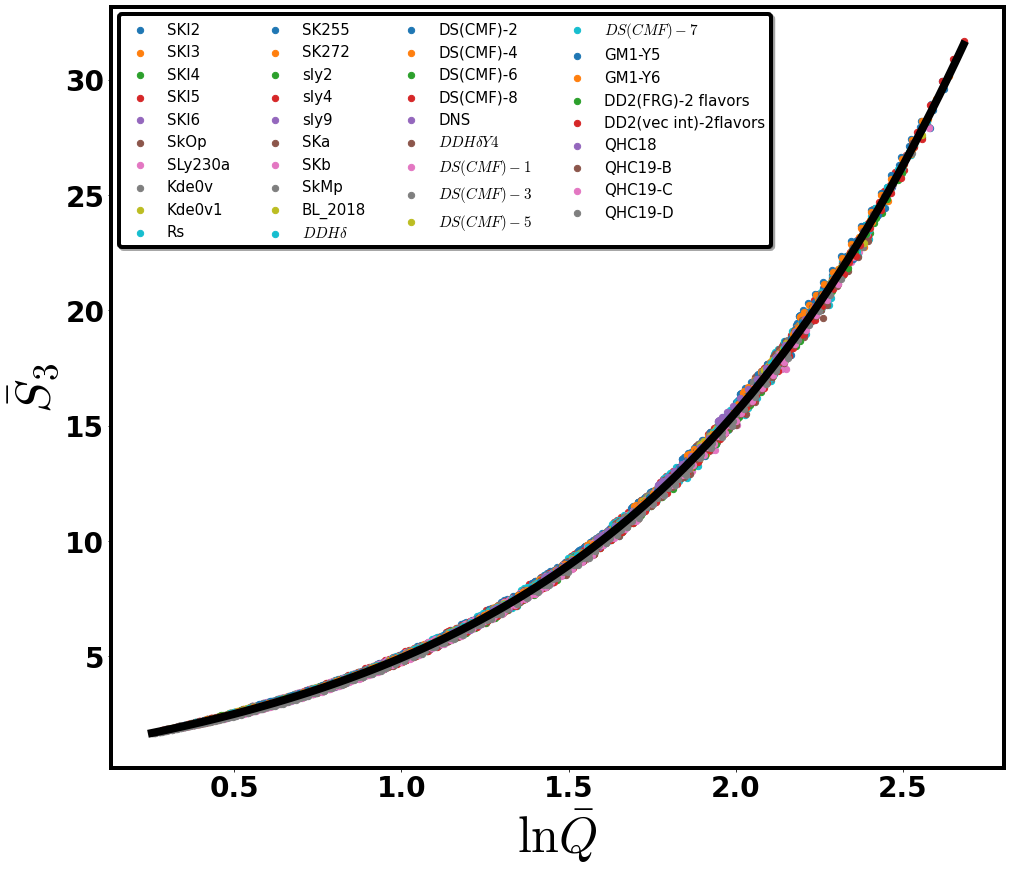
Investigation of the correlation \(\bar{S_3}=f(\chi,\bar{Q})\)#
df7 = {'x': x_spin, 'Qbar': quadr, 'S3bar':S3_bar}
df7=pd.DataFrame(data=df7, index=None, columns=None, dtype=None, copy=False)
df7.reset_index(drop=True, inplace=True)
Cross validation statistical metrics and results for different ‘pol degrees’ \(\kappa\)#
#cv_results = c_val_performace_results_for_k(df7,x='x',y='Qbar',z='S3bar')
#cv_results
pd.read_csv(r"LOOCV_results/S3bar_chi_Qbar_cv_scores.txt", sep=' ')
# best functional form form for pol_degree = 3
| MAE | Max_Error | MSE | d(%) | MAPE(%) | Explained_Variance | k | |
|---|---|---|---|---|---|---|---|
| 0 | 0.060527 | 0.627345 | 0.007913 | 4.882781 | 0.899585 | 1.0 | 2.0 |
| 1 | 0.059563 | 0.661218 | 0.007800 | 3.289495 | 0.864612 | 1.0 | 3.0 |
| 2 | 0.058844 | 0.666478 | 0.007740 | 3.386168 | 0.841361 | 1.0 | 4.0 |
| 3 | 0.058701 | 0.672730 | 0.007725 | 3.417933 | 0.833712 | 1.0 | 5.0 |
| 4 | 0.058585 | 0.680666 | 0.007706 | 3.458255 | 0.833739 | 1.0 | 6.0 |
| 5 | 0.058418 | 0.669064 | 0.007681 | 3.423339 | 0.828776 | 1.0 | 7.0 |
Linear Regression at training data#
df7['S3bar_model'] = Regression_function(df7,x = 'x',y= 'Qbar' ,z='S3bar', pol_degree=3, x_power = 'x',y_power='Qbar')[0]
#df7['S3bar_model']
\(R^2\) - quality index#
Regression_function(df7,x = 'x',y= 'Qbar' ,z='S3bar', pol_degree=3, x_power = 'x',y_power='Qbar')[1]
0.9997499756233522
Evaluation functions at training data#
relative_training_error_plot(df7, 'S3bar' , 'S3bar_model', xlabel='Data', ylabel=r'$(\Delta\bar{S_3}/\bar{S_3})\times 100\%$')
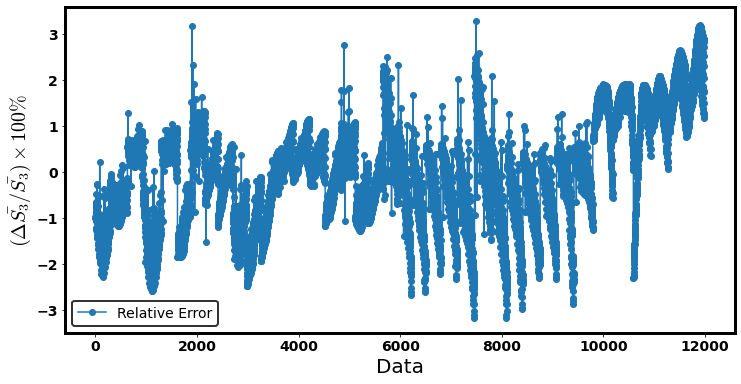
<AxesSubplot:xlabel='Data', ylabel='$(\\Delta\\bar{S_3}/\\bar{S_3})\\times 100\\%$'>
training_error_funct(df7, 'S3bar' , 'S3bar_model')
| train_Max_Error | d_max_training(%) | MAPE_taining(%) | |
|---|---|---|---|
| 0 | 0.650781 | 3.277124 | 0.863946 |
training_relative_error_hist(df7, 'S3bar', 'S3bar_model',
                             r'$(\Delta\bar{S_3}/\bar{S_3})\times 100\%$', r'Rotating Neutron Star models',n_bins=20,
                             x1_lim=-10, x2_lim=10)
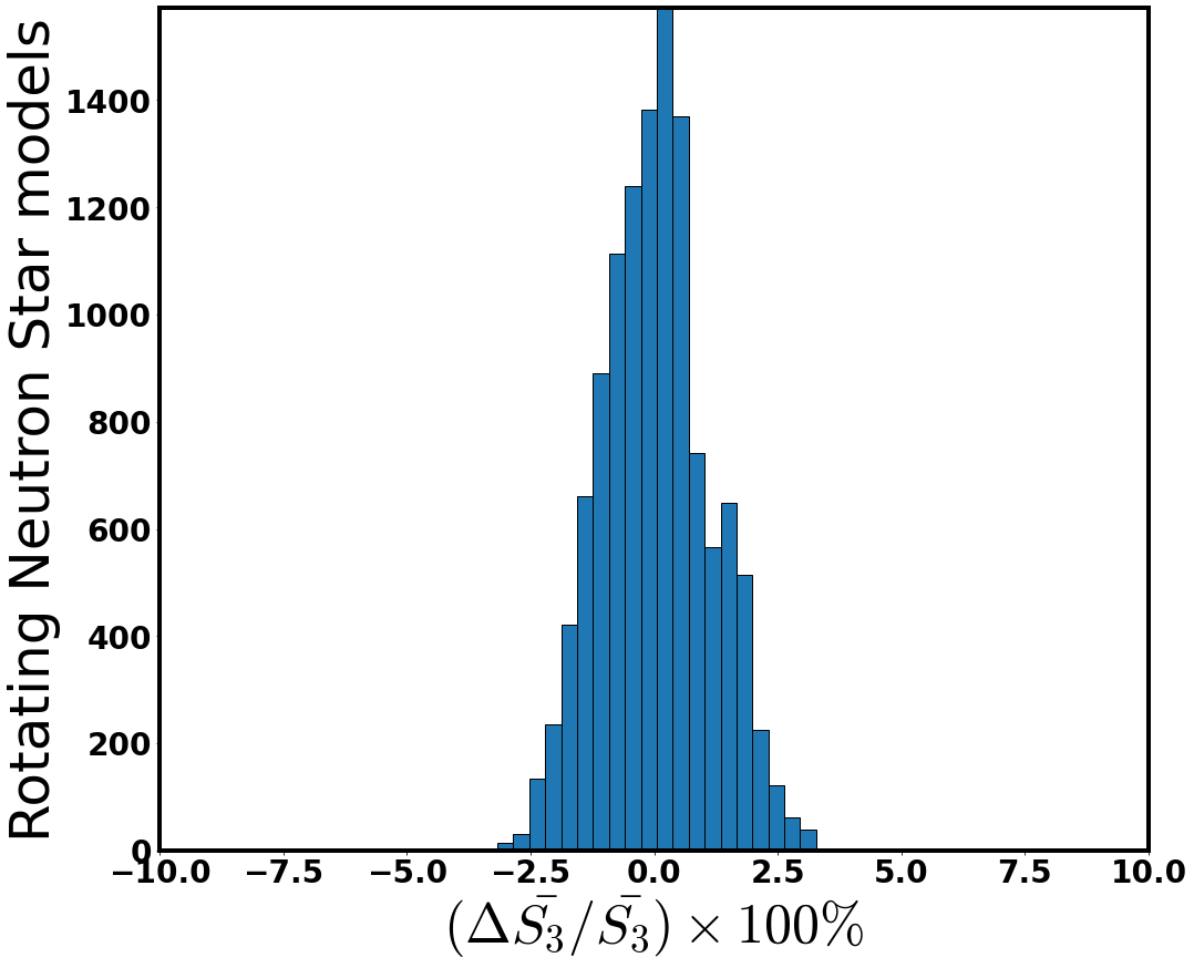
Error distribution at space#
relative_error_space_distribution(df7, 'x' , 'Qbar' ,'S3bar','S3bar_model' ,
                                  r'$\chi$',r'$\bar{Q}$', r'$(|\Delta\bar{S_3}|/\bar{S_3})\times 100\%$', view2=250)
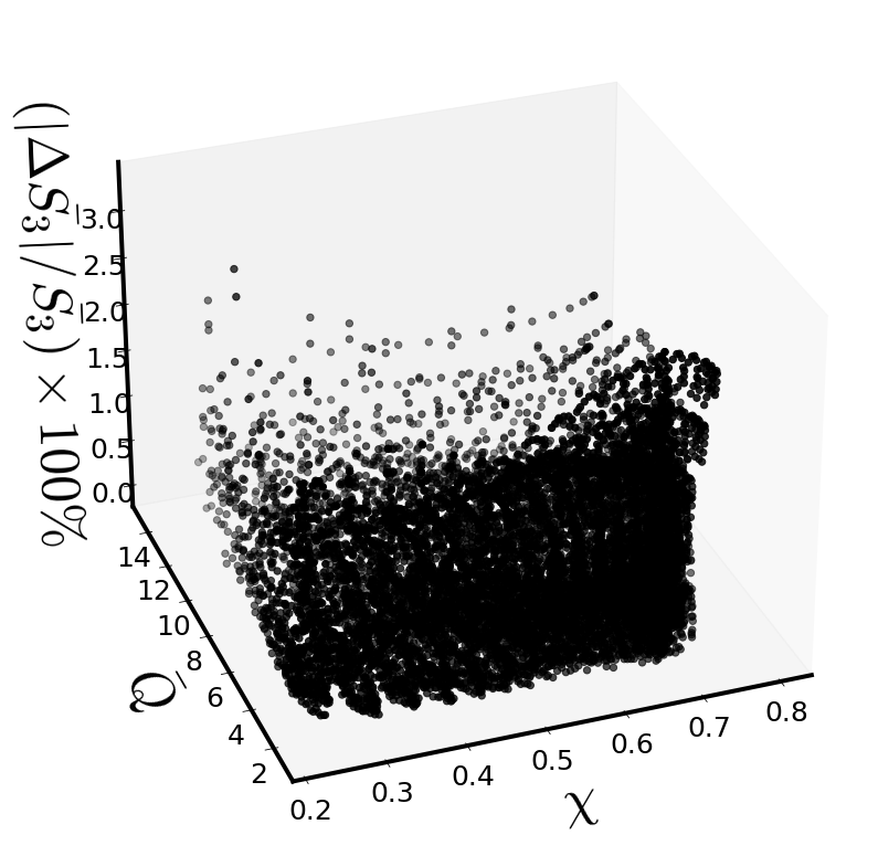
Best Model’s optimizers-coefficients#
# model's intercept
l_00 = Regression_function(df7,x = 'x',y= 'Qbar' ,z='S3bar', pol_degree=3, x_power = 'x',y_power='Qbar')[2]
# other model's coefficients
l_nm = Regression_function(df7,x = 'x',y= 'Qbar' ,z='S3bar', pol_degree=3, x_power = 'x',y_power='Qbar')[3]
# Results stored in data frame
coef7=pd.DataFrame(l_nm,columns=["coef"])
#Regression_function(df7,x = 'x',y= 'Qbar' ,z='S3bar', pol_degree=3, x_power = 'x',y_power='Qbar')[4]
powers7 = Regression_function(df7,x = 'x',y= 'Qbar' ,z='S3bar', pol_degree=3,
                              x_power = 'x',y_power='Qbar')[5]
#powers7
def S3_bar_x_qbar_funct(x,qbar):
    results=0
    for i in range(0,len(powers7)):
        results += (coef7["coef"][i]*x**(powers7["x"][i])*qbar**(powers7["Qbar"][i]))

    return l_00 + results
Regression Function#
S3_bar_x_qbar_funct(chi_s,qbar_s).collect(chi_s)
\[\displaystyle - 1.66542035797461 \chi^{3} + \chi^{2} \left(0.0445526492805266 {\left(\bar{Q}\right)} + 2.60994286681048\right) + \chi \left(- 0.00988459866794515 {\left(\bar{Q}\right)}^{2} + 0.182919172134776 {\left(\bar{Q}\right)} - 1.3965113048512\right) + 2.84184495151774 \cdot 10^{-5} {\left(\bar{Q}\right)}^{3} + 0.00467744159847946 {\left(\bar{Q}\right)}^{2} + 2.17171530010352 {\left(\bar{Q}\right)} - 1.00461158164299\]
Fitting Surface compared to data#
x7 = mesh_grid_funct(df7,x_name = 'x', y_name = 'Qbar')[0]
y7 = mesh_grid_funct(df7,x_name = 'x', y_name = 'Qbar')[1]
Z_7 = S3_bar_x_qbar_funct(x7,y7)
Surface_plot_funct_2(eos_data, 'x','q_tilde_GH','S3_bar_GH', xlabel=r'$\chi$',ylabel=r'$\bar{Q}$',zlabel=r'$\bar{S}_3$',
                     view2=250, n_col=5, border_axes=8, X=x7,Y=y7,Z=Z_7, l_w=1.5)
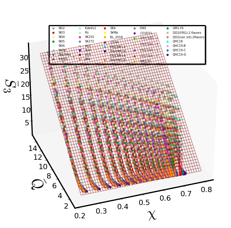
Investigation of the \(\bar{S_3}=f(\sigma,\bar{Q})\) parameterization#
df8 = {'C':C,'sigma': sigma, 'Qbar': quadr, 'S3bar':S3_bar}
df8=pd.DataFrame(data=df8, index=None, columns=None, dtype=None, copy=False)
df8.reset_index(drop=True, inplace=True)
#df8
Cross validation statistical metrics and results for different ‘pol degrees’ \(\kappa\)#
#cv_results = c_val_performace_results_for_k(df8,x='sigma',y='Qbar',z='S3bar')
#cv_results
pd.read_csv(r"LOOCV_results/S3bar_sigma_Qbar_cv_scores.txt", sep=' ')
#best functional form form for pol_degree = 3
| MAE | Max_Error | MSE | d(%) | MAPE(%) | Explained_Variance | k | |
|---|---|---|---|---|---|---|---|
| 0 | 0.056968 | 0.661739 | 0.007081 | 3.362094 | 0.850004 | 1.0 | 2.0 |
| 1 | 0.056009 | 0.646545 | 0.006982 | 3.207825 | 0.812496 | 1.0 | 3.0 |
| 2 | 0.055378 | 0.647638 | 0.006930 | 3.290447 | 0.791042 | 1.0 | 4.0 |
| 3 | 0.055381 | 0.659184 | 0.006929 | 3.349112 | 0.793840 | 1.0 | 5.0 |
| 4 | 0.055643 | 0.686659 | 0.006977 | 3.488705 | 0.802122 | 1.0 | 6.0 |
| 5 | 0.055268 | 0.660194 | 0.006911 | 3.354241 | 0.787729 | 1.0 | 7.0 |
Linear Regression at training data#
df8['S3bar_model'] = Regression_function(df8,x = 'sigma',y= 'Qbar' ,z='S3bar', pol_degree=3, x_power = 'sigma',y_power='Qbar')[0]
#df8['S3bar_model']
\(R^2\) - quality index#
Regression_function(df8,x = 'sigma',y= 'Qbar' ,z='S3bar', pol_degree=3, x_power = 'sigma',y_power='Qbar')[1]
0.99977618120854
Evaluation functions at training data#
relative_training_error_plot(df8, 'S3bar' , 'S3bar_model', xlabel='Data', ylabel=r'$(\Delta\bar{S_3}/\bar{S_3})\times 100\%$')
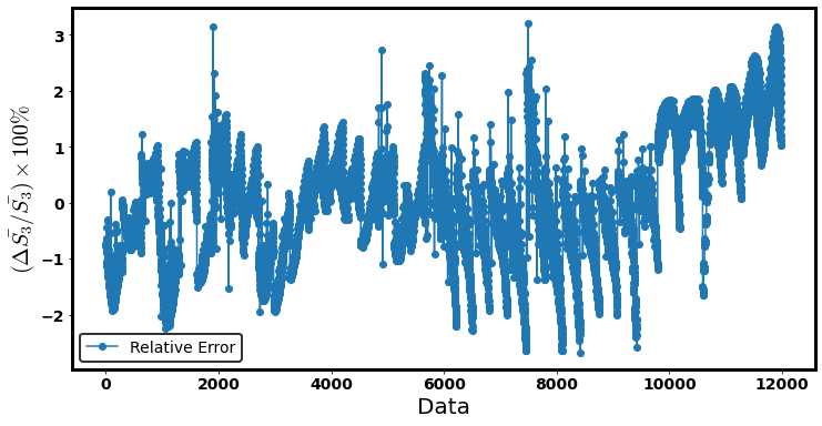
<AxesSubplot:xlabel='Data', ylabel='$(\\Delta\\bar{S_3}/\\bar{S_3})\\times 100\\%$'>
training_error_funct(df8, 'S3bar' , 'S3bar_model')
| train_Max_Error | d_max_training(%) | MAPE_taining(%) | |
|---|---|---|---|
| 0 | 0.637849 | 3.198451 | 0.811844 |
training_relative_error_hist(df8, 'S3bar', 'S3bar_model',
                             r'$(\Delta\bar{S_3}/\bar{S_3})\times 100\%$', r'Rotating Neutron Star models',n_bins=20,
                             x1_lim=-5, x2_lim=5)
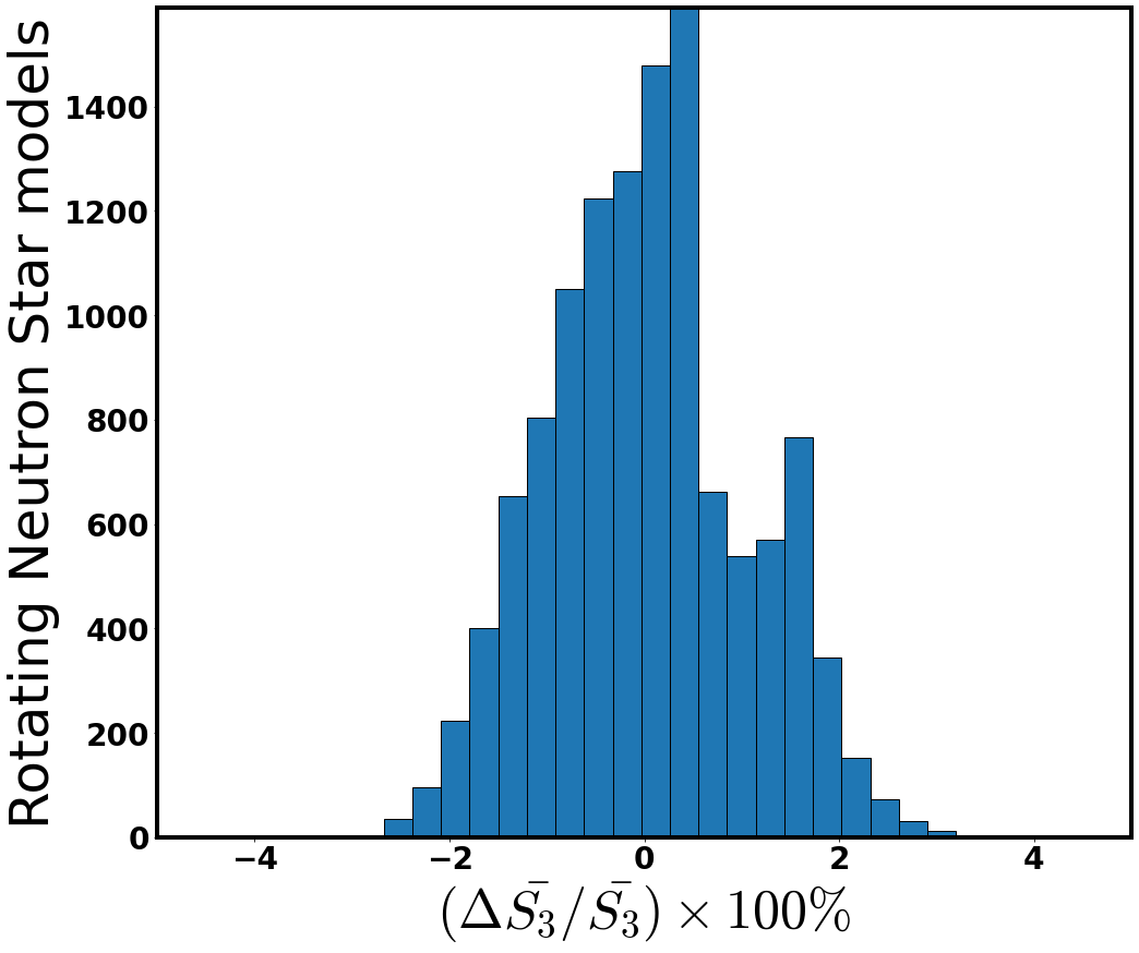
Error distribution at space#
relative_error_space_distribution(df8, 'sigma' , 'Qbar' ,'S3bar','S3bar_model' ,
                                  r'$\sigma$',r'$\bar{Q}$', r'$(|\Delta\bar{S_3}|/\bar{S_3})\times 100\%$', view2=250)
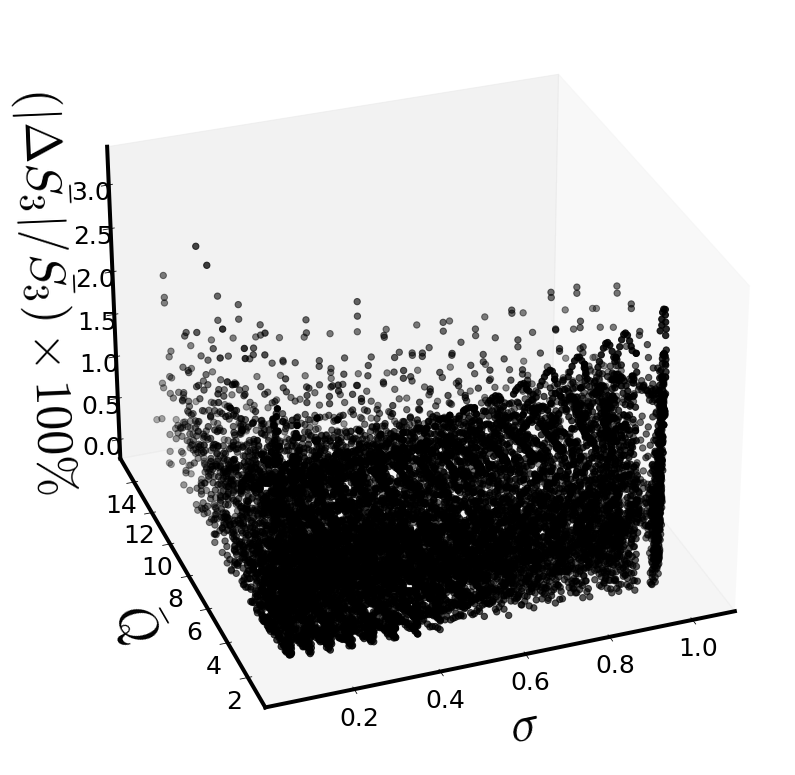
Indicative relative deviations?#
variance_of_errors(df=df8,reference_deviation = 3,z = df8['S3bar'],z_model=df8['S3bar_model'])[['sigma','C','Qbar']]
| sigma | C | Qbar | |
|---|---|---|---|
| 1903 | 0.073549 | 0.125575 | 8.592419 |
| 7494 | 0.071371 | 0.119406 | 9.600227 |
| 11864 | 0.945668 | 0.265572 | 1.481129 |
| 11881 | 0.943281 | 0.273306 | 1.423748 |
| 11898 | 0.938454 | 0.279018 | 1.386415 |
| 11915 | 0.934910 | 0.284592 | 1.350979 |
| 11932 | 0.932490 | 0.289579 | 1.319839 |
variance_of_errors(df=df8,reference_deviation = 3,z = df8['S3bar'],z_model=df8['S3bar_model'])[['sigma','C','Qbar']].min()
sigma    0.071371
C        0.119406
Qbar     1.319839
dtype: float64
variance_of_errors(df=df8,reference_deviation = 3,z = df8['S3bar'],z_model=df8['S3bar_model'])[['sigma','C','Qbar']].max()
sigma    0.945668
C        0.289579
Qbar     9.600227
dtype: float64
Best Model’s optimizers-coefficients#
# model's intercept
p_00 = Regression_function(df8,x = 'sigma',y= 'Qbar' ,z='S3bar', pol_degree=3, x_power = 'sigma',y_power='Qbar')[2]
# Other model's coefficient
p_nm = Regression_function(df8,x = 'sigma',y= 'Qbar' ,z='S3bar', pol_degree=3, x_power = 'sigma',y_power='Qbar')[3]
# Results stored in data frame
coef8=pd.DataFrame(p_nm,columns=["coef"])
#coef8
#Regression_function(df8,x = 'sigma',y= 'Qbar' ,z='S3bar', pol_degree=3, x_power = 'sigma',y_power='Qbar')[4]
powers8 = Regression_function(df8,x = 'sigma',y= 'Qbar' ,z='S3bar', pol_degree=3,
x_power = 'sigma',y_power='Qbar')[5]
#powers8
def S3_bar_sigma_qbar_funct(sigma,qbar):
results=0
for i in range(0,len(powers8)):
results += (coef8["coef"][i]*sigma**(powers8["sigma"][i])*qbar**(powers8["Qbar"][i]))
return p_00 + results
Regression Function#
S3_bar_sigma_qbar_funct(sigma_s,qbar_s).collect(sigma_s)
\[\displaystyle - 0.0472956768901432 \sigma^{3} + \sigma^{2} \left(0.109773896571624 - 0.0635523821185354 {\left(\bar{Q}\right)}\right) + \sigma \left(- 0.00224621909234078 {\left(\bar{Q}\right)}^{2} + 0.167367997674104 {\left(\bar{Q}\right)} - 0.0929986624617679\right) + 0.000146260584131711 {\left(\bar{Q}\right)}^{3} - 0.000193943103910888 {\left(\bar{Q}\right)}^{2} + 2.22430535168964 {\left(\bar{Q}\right)} - 1.24418312578412\]
Fitting Surface compared to data#
x8 = mesh_grid_funct(df8,x_name = 'sigma', y_name = 'Qbar')[0]
y8 = mesh_grid_funct(df8,x_name = 'sigma', y_name = 'Qbar')[1]
Z_8 = S3_bar_sigma_qbar_funct(x8,y8)
Surface_plot_funct_2(eos_data, 'sigma','q_tilde_GH','S3_bar_GH', xlabel=r'$\sigma$',ylabel=r'$\bar{Q}$',zlabel=r'$\bar{S}_3$',
view2=250, n_col=5, border_axes=1, X=x8,Y=y8,Z=Z_8, l_w=1.5)
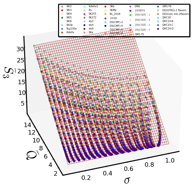
Investigation of the \(\bar{S_3}=f(\mathcal{E},\bar{Q})\) parameterization#
df9 = {'T/W': T_over_W, 'Qbar': quadr, 'lnQbar':np.log(quadr) ,'S3bar':S3_bar}
df9=pd.DataFrame(data=df9, index=None, columns=None, dtype=None, copy=False)
df9.reset_index(drop=True, inplace=True)
#df9
Cross validation statistical metrics and results for different ‘pol degrees’ \(\kappa\)#
#cv_results = c_val_performace_results_for_k(df9,x='T/W',y='Qbar',z='S3bar')
#cv_results
pd.read_csv(r"LOOCV_results/S3bar_T_W_Qbar_cv_scores.txt", sep=' ')
# best functional form form for pol_degree = 2
| MAE | Max_Error | MSE | d(%) | MAPE(%) | Explained_Variance | k | |
|---|---|---|---|---|---|---|---|
| 0 | 0.059652 | 0.640182 | 0.007831 | 3.252569 | 0.865831 | 1.0 | 2.0 |
| 1 | 0.059436 | 0.651122 | 0.007804 | 3.308149 | 0.856899 | 1.0 | 3.0 |
| 2 | 0.058926 | 0.663255 | 0.007762 | 3.369795 | 0.840436 | 1.0 | 4.0 |
| 3 | 0.058819 | 0.668872 | 0.007753 | 3.398335 | 0.836501 | 1.0 | 5.0 |
| 4 | 0.058707 | 0.675960 | 0.007739 | 3.434344 | 0.834671 | 1.0 | 6.0 |
| 5 | 0.058748 | 0.676389 | 0.007728 | 3.452384 | 0.835360 | 1.0 | 7.0 |
Linear Regression at training data#
df9['S3bar_model'] = Regression_function(df9,x = 'T/W',y= 'Qbar' ,z='S3bar', pol_degree=2, x_power = 'T/w',y_power='Qbar')[0]
#df9['S3bar_model']
\(R^2\) - quality index#
Regression_function(df9,x = 'T/W',y= 'Qbar' ,z='S3bar', pol_degree=2, x_power = 'T/w',y_power='Qbar')[1]
0.9997485030152768
Evaluation functions at training data#
relative_training_error_plot(df9, 'S3bar' , 'S3bar_model', xlabel='Data', ylabel=r'$(\Delta\bar{S_3}/\bar{S_3})\times 100\%$')
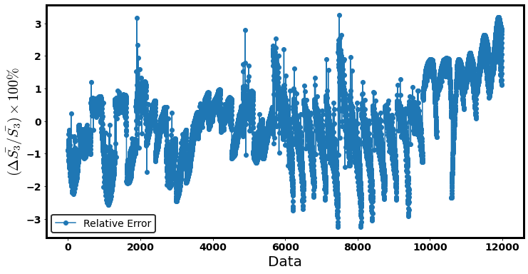
<AxesSubplot:xlabel='Data', ylabel='$(\\Delta\\bar{S_3}/\\bar{S_3})\\times 100\\%$'>
training_error_funct(df9, 'S3bar' , 'S3bar_model')
| train_Max_Error | d_max_training(%) | MAPE_taining(%) | |
|---|---|---|---|
| 0 | 0.639211 | 3.247635 | 0.865414 |
training_relative_error_hist(df9, 'S3bar', 'S3bar_model',
r'$(\Delta\bar{S_3}/\bar{S_3})\times 100\%$', r'Rotating Neutron Star models',n_bins=20,
x1_lim=-10, x2_lim=10)
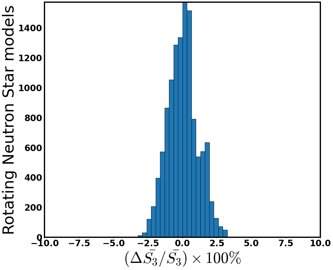
Error distribution at space#
relative_error_space_distribution(df9, 'T/W' , 'Qbar' ,'S3bar','S3bar_model' ,
r'$\mathcal{E}$',r'$\bar{Q}$', r'$(|\Delta\bar{S_3}|/\bar{S_3})\times 100\%$', view2=250)
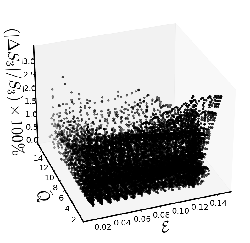
Best Model’s optimizers-coefficients#
# model's intercept
q_00 = Regression_function(df9,x = 'T/W',y= 'Qbar' ,z='S3bar', pol_degree=2, x_power = 'T/w',y_power='Qbar')[2]
# Other model's coefficients
q_nm = Regression_function(df9,x = 'T/W',y= 'Qbar' ,z='S3bar', pol_degree=2, x_power = 'T/w',y_power='Qbar')[3]
# Results stored in data frame
coef9=pd.DataFrame(q_nm,columns=["coef"])
#coef9
#Regression_function(df9,x = 'T/W',y= 'Qbar' ,z='S3bar', pol_degree=2, x_power = 'T/w',y_power='Qbar')[4]
powers9 = Regression_function(df9,x = 'T/W',y= 'Qbar' ,z='S3bar', pol_degree=2,
x_power = 'T/w',y_power='Qbar')[5]
#powers9
def S3_bar_tw_qbar_funct(t_w,qbar):
results=0
for i in range(0,len(powers9)):
results += (coef9["coef"][i]*t_w**(powers9["T/w"][i])*qbar**(powers9["Qbar"][i]))
return q_00 + results
Regression Function#
S3_bar_tw_qbar_funct(TW_s,qbar_s).collect(TW_s)
\[\displaystyle - 1.97597308366342 \mathcal{E}^{2} + \mathcal{E} \left(0.758132049336647 {\left(\bar{Q}\right)} + 0.0131524970103299\right) + 0.00230042408645165 {\left(\bar{Q}\right)}^{2} + 2.21372807212532 {\left(\bar{Q}\right)} - 1.24075686382165\]
Fitting Surface compared to data#
x9 = mesh_grid_funct(df9,x_name = 'T/W', y_name = 'Qbar')[0]
y9 = mesh_grid_funct(df9,x_name = 'T/W', y_name = 'Qbar')[1]
Z_9 = S3_bar_tw_qbar_funct(x9,y9)
Surface_plot_funct_2(eos_data, 'T/W','q_tilde_GH','S3_bar_GH', xlabel=r'$\mathcal{E}$',ylabel=r'$\bar{Q}$',zlabel=r'$\bar{S}_3$',
view2=250, n_col=5, border_axes=8, X=x9,Y=y9,Z=Z_9, l_w=2.5)
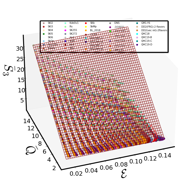
Investigation of the \(\bar{S}_3 = \bar{S_3}(M\times \tilde{f}, \bar{Q})\) parameterization#
df10 = {'C':C,'x':x_spin,'sigma':sigma,'M*f/c':M_x_f, "R*f/c": R_x_f,'qbar': quadr, 'ln(qbar)':np.log(quadr),'Ibar':I_bar,'S3bar':S3_bar}
df10 = pd.DataFrame(data=df10, index=None, columns=None, dtype=None, copy=False)
df10.reset_index(drop=True, inplace=True)
#df10
Cross validation statistical metrics and results for different ‘pol degrees’ \(\kappa\)#
#cv_results = c_val_performace_results_for_k(df10,x='M*f/c',y='qbar',z='S3bar')
#cv_results
pd.read_csv(r"LOOCV_results/S3bar_Mf_Qbar_cv_scores.txt", sep=' ')
# best functional form form for pol_degree = 3
| MAE | Max_Error | MSE | d(%) | MAPE(%) | Explained_Variance | k | |
|---|---|---|---|---|---|---|---|
| 0 | 0.064985 | 0.758767 | 0.009132 | 4.223056 | 1.008774 | 1.0 | 2.0 |
| 1 | 0.059871 | 0.576134 | 0.008043 | 3.161201 | 0.856989 | 1.0 | 3.0 |
| 2 | 0.058563 | 0.646826 | 0.007616 | 3.286323 | 0.848144 | 1.0 | 4.0 |
| 3 | 0.057931 | 0.690482 | 0.007556 | 3.508127 | 0.824260 | 1.0 | 5.0 |
| 4 | 0.057808 | 0.664039 | 0.007505 | 3.373780 | 0.822430 | 1.0 | 6.0 |
| 5 | 0.057765 | 0.656607 | 0.007503 | 3.336018 | 0.821855 | 1.0 | 7.0 |
Linear Regression at training data#
df10['S3bar_model'] = Regression_function(df10,x = 'M*f/c',y= 'qbar' ,z='S3bar', pol_degree=3, x_power = 'M*f/c',y_power='ln(qbar)')[0]
#df10['S3bar_model']
\(R^2\) - quality index#
Regression_function(df10,x = 'M*f/c',y= 'ln(qbar)' ,z='S3bar', pol_degree=3, x_power = 'M*f/c',y_power='Qbar')[1]
0.9997253781156649
Evaluation functions at training data#
relative_training_error_plot(df10, 'S3bar' , 'S3bar_model', xlabel='Data', ylabel=r'$(\Delta\bar{S_3}/\bar{S_3})\times 100\%$')
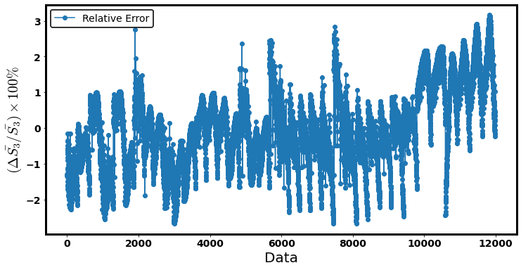
<AxesSubplot:xlabel='Data', ylabel='$(\\Delta\\bar{S_3}/\\bar{S_3})\\times 100\\%$'>
training_error_funct(df10, 'S3bar' , 'S3bar_model')
| train_Max_Error | d_max_training(%) | MAPE_taining(%) | |
|---|---|---|---|
| 0 | 0.569945 | 3.158913 | 0.856301 |
training_relative_error_hist(df10, 'S3bar', 'S3bar_model',
r'$(\Delta\bar{S_3}/\bar{S_3})\times 100\%$', r'Rotating Neutron Star models',n_bins=20,
x1_lim=-5, x2_lim=5)
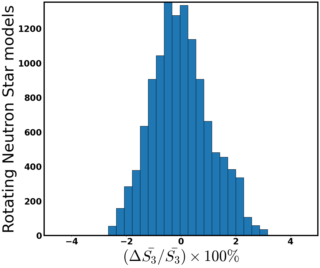
Error distribution at space#
relative_error_space_distribution(df10, 'M*f/c' , 'qbar' ,'S3bar','S3bar_model' ,
r'$M\times f/c$',r'$\bar{Q}$', r'$(|\Delta\bar{S_3}|/\bar{S_3})\times 100\%$',
view2=230)
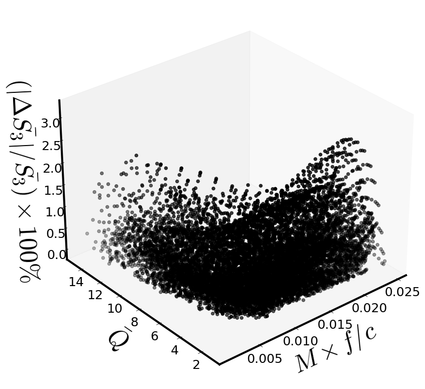
Indicative relative deviations?#
#variance_of_errors(df=df10,reference_deviation = 3,z = df10['S3bar'],z_model=df10['S3bar_model'])[['x','sigma','M*f/c','C','qbar']]
len(variance_of_errors(df=df10,reference_deviation = 3,z = df10['S3bar'],z_model=df10['S3bar_model'])[['x','sigma','M*f/c','C','qbar']])
19
variance_of_errors(df=df10,reference_deviation = 3,z = df10['S3bar'],z_model=df10['S3bar_model'])[['x','sigma','M*f/c','C','qbar']].min()
x 0.638905
sigma 0.604954
M*f/c 0.016164
C 0.229705
qbar 1.546866
dtype: float64
variance_of_errors(df=df10,reference_deviation = 3,z = df10['S3bar'],z_model=df10['S3bar_model'])[['x','sigma','M*f/c','C','qbar']].max()
x 0.718153
sigma 0.961997
M*f/c 0.020257
C 0.270161
qbar 1.886485
dtype: float64
Best Model’s optimizers-coefficients#
# model's intercept
w_00 = Regression_function(df10,x = 'M*f/c',y= 'qbar' ,z='S3bar', pol_degree=3, x_power = 'M*f/c',y_power='Qbar')[2]
# other model's coefficient
w_nm = Regression_function(df10,x = 'M*f/c',y= 'qbar' ,z='S3bar', pol_degree=3, x_power = 'M*f/c',y_power='Qbar')[3]
# Results stored in data frame
coef10=pd.DataFrame(w_nm,columns=["coef"])
#coef10
#Regression_function(df10,x = 'M*f/c',y= 'qbar' ,z='S3bar', pol_degree=3, x_power = 'M*f/c',y_power='Qbar')[4]
powers10 = Regression_function(df10,x = 'M*f/c',y= 'qbar' ,z='S3bar',
pol_degree=3, x_power = 'M*f/c',y_power='Qbar')[5]
#powers10
def S3_bar_Mf_qbar(x,y):
results=0
for i in range(0,len(powers10)):
results+=(coef10["coef"][i]*x**(powers10["M*f/c"][i])*y**(powers10["Qbar"][i]))
return w_00 + results
Fitting Surface compared to data#
x10 = mesh_grid_funct(df10,x_name = 'M*f/c', y_name = 'qbar')[0]
y10 = mesh_grid_funct(df10,x_name = 'M*f/c', y_name = 'qbar')[1]
Z_10 = S3_bar_Mf_qbar(x10,y10)
Surface_plot_funct_2(eos_data, 'M*f/c','q_tilde_GH','S3_bar_GH', xlabel=r'$M\times \tilde{f}$',ylabel=r'$\bar{Q}$',
zlabel=r'$\bar{S_3}$',
view2=230, n_col=5, border_axes=1, X=x10,Y=y10,Z=Z_10, l_w=1.5)
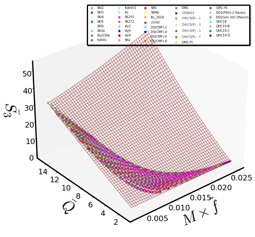
Correlation Matrix#
dictionary_values = {r'$C$': df['C'].to_numpy(),
r'$\mathcal{K}$': (1/df['C']).to_numpy(),
r'$M\times f/c$': df10["M*f/c"].to_numpy(),
r'$R_{eq}\times f/c$': df10["R*f/c"].to_numpy(),
r'$\chi$': df2['x'].to_numpy(),
r'$\sigma$': df3['sigma'].to_numpy(),
r'$T/|W|$': df9['T/W'].to_numpy(),
r'$M\times f/\chi$': df4_b['M*f/x'].to_numpy(),
r'$\bar{I}$': df5['Ibar'].to_numpy(),
r'$\bar{Q}$': df3['qbar'].to_numpy(),
r'$\ln(\bar{Q})$': df6['ln(qbar)'].to_numpy(),
r'$\bar{S_3}$': df6['S3bar'].to_numpy()
}
list_names = [r'$C$',r'$\mathcal{K}$',r'$M\times f/c$',r'$R_{eq}\times f/c$',r'$\chi$' ,r'$\sigma$',r'$T/|W|$',
r'$M\times f/\chi$',r'$\bar{I}$',r'$\bar{Q}$',r'$\ln(\bar{Q})$', r'$\bar{S_3}$']
corr_matrix_funct(dict_values = dictionary_values, col_names_list = list_names)