Ranking Statistic Analysis of O3a Month 2 Triggers using AresGW Model 1

AresGW ACME training session

Alexandra Eleni Koloniari

Aristotle University of Thessaloniki

import numpy as np
import h5py
import matplotlib.pyplot as plt

Ranking statistic \(R_s\)

In this notebook the ranking statistic is computed as:

rs = -np.log10(1.0 - stat[:] + 1e-16)

This definition follows the statistic used in:

A. E. Koloniari et al., “New Gravitational Wave Discoveries Enabled by Machine Learning” (2024)

The small constant 1e-16 is added to prevent numerical issues when stat → 1, which would otherwise lead to log10(0).

READ THE TRIGGERS FILE

filename = 'AresGW-model1-O3a-data-m2.hdf'

f =  h5py.File(filename,'r')

f.keys()

<KeysViewHDF5 ['stat', 'time', 'var']>

f_stat = f.get('stat')
f_time = f.get('time')
f_var= f.get('var')

stat = f_stat[()]
stat = -np.log10(1.0-stat[:]+1e-16)
time = f_time[()]
var = f_var[()]

# First trigger time
time[0]

1240758022.925

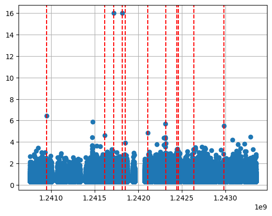
MERGER TIMES OF EVENTS IN SECOND MONTH OF O3a

# List with the GPS times of all detected events in the second month of O3a
tc_list = [
    1240944862.3,
    1241719652.4,
    1241816086.8,
    1241852074.8,
    1242107479.8,
    1242315362.4,
    1242442967.4,
    1242459857.5,
    1242984073.8,
    1241614563.9,
    1242637191.4
]
# List with the corresponding names and Catalogs
gw_name_list = [
    "GW190503_185404 (GWTC)",  # 1240944862.3
    "GW190512_180714 (GWTC)",  # 1241719652.4
    "GW190513_205428 (GWTC)",  # 1241816086.8
    "GW190514_065416 (GWTC)",  # 1241852074.8
    "GW190517_055101 (GWTC)",  # 1242107479.8
    "GW190519_153544 (GWTC)",  # 1242315362.4
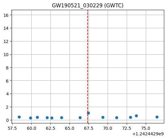
    "GW190521_030229 (GWTC)",  # 1242442967.4 
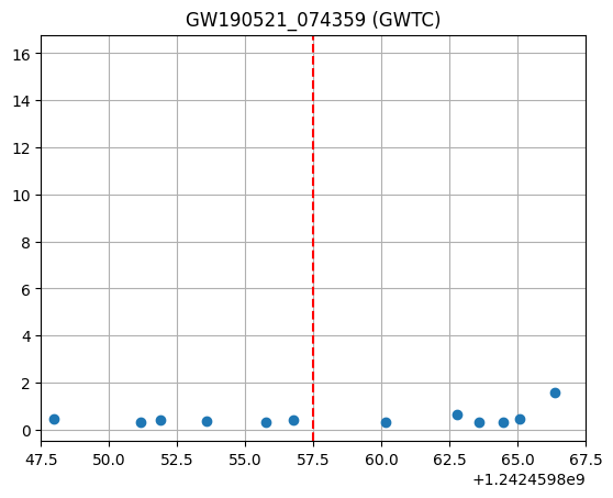
    "GW190521_074359 (GWTC)",  # 1242459857.5
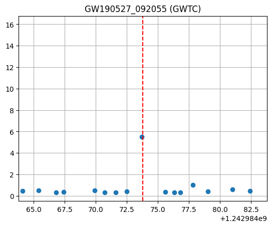
    "GW190527_092055 (GWTC)",  # 1242984073.8
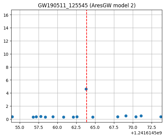
    "GW190511_125545 (AresGW model 2)", #1241614563.9
    "GW190523_085933 (AresGW model 2)"  #1242637191.4
]

graph, plot = plt.subplots(1)

plot.plot(np.array(time), np.array(stat), 'o')
plt.grid()

for tc in tc_list:
    plt.axvline(x=tc, color='r', linestyle='dashed')

plt.show()

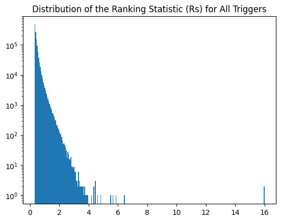
# Histogram of the ranking statistic (Rs) for all triggers
# Includes both noise triggers and triggers associated with GW events
count, bins, ignored = plt.hist(np.array(stat), 300)

plt.yscale('log')  # Log scale to better visualize the distribution tail
plt.title('Distribution of the Ranking Statistic (Rs) for All Triggers')

plt.show()

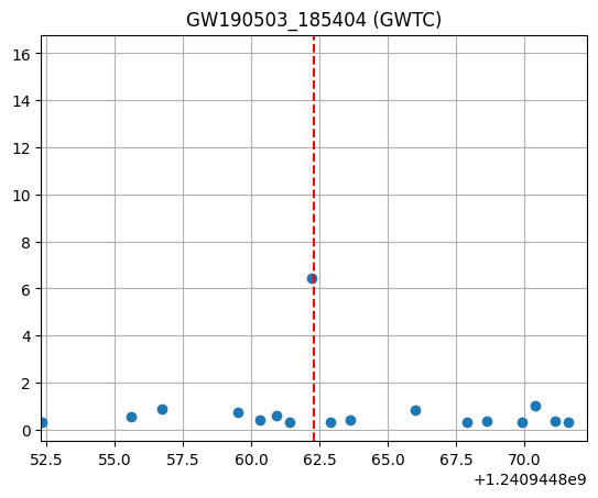
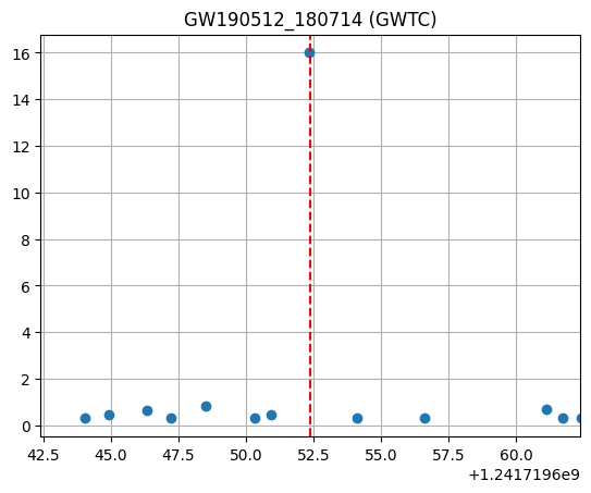
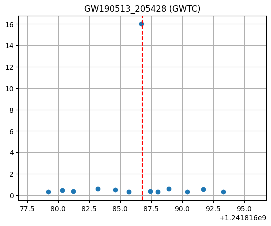
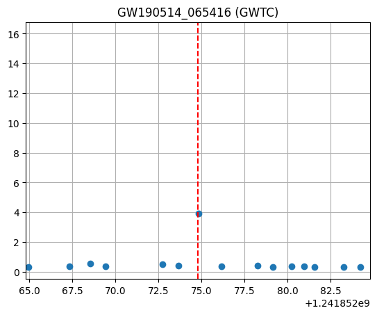
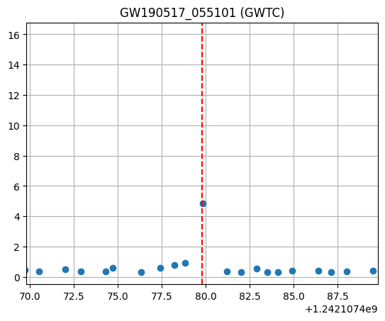
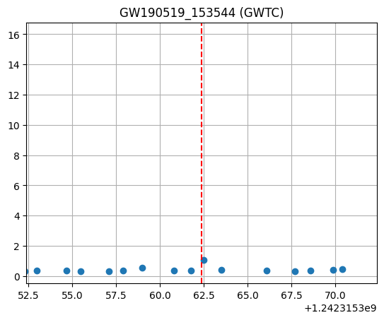
# Rs for each event and its nearby noise
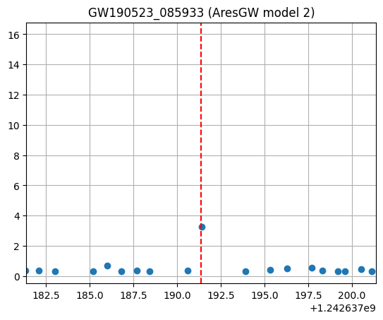
for tc, name in zip(tc_list, gw_name_list):

    fig, ax = plt.subplots()
    ax.plot(time, stat, 'o')

    ax.axvline(tc, color='r', linestyle='dashed')
    ax.set_xlim(tc-10, tc+10)

    ax.set_title(name)
    ax.grid()

    plt.show()

print("Total number of triggers (noise and events) above different thresholds:")
rs = np.array(stat)

count_3 = np.sum(rs > 3)
count_7 = np.sum(rs > 7)
count_10 = np.sum(rs > 10)
count_16 = np.sum(rs == 16)

print(f"Number of triggers with Rs > 3  : {count_3}")
print(f"Number of triggers with Rs > 7  : {count_7}")
print(f"Number of triggers with Rs > 10 : {count_10}")
print(f"Number of triggers with Rs = 16 : {count_16}")

Total number of triggers (noise and events) above different thresholds:
Number of triggers with Rs > 3  : 66
Number of triggers with Rs > 7  : 2
Number of triggers with Rs > 10 : 2
Number of triggers with Rs = 16 : 2

print("Rs of each event in m2 is:")

for tc, name in zip(tc_list, gw_name_list):

    # Different windows
    a = np.where((time < tc + 0.5) & (time > tc - 0.5))[0]
    b = np.where((time < tc + 0.3) & (time > tc - 0.5))[0]
    c = np.where((time < tc + 0.5) & (time > tc - 0.3))[0]

    if len(a) == 1:
        trigger_index = int(a[0])
    elif len(b) == 1:
        trigger_index = int(b[0])
    elif len(c) == 1:
        trigger_index = int(c[0])
    else:
        continue

    print(name, stat[trigger_index])

Rs of each event in m2 is:
GW190503_185404 (GWTC) 6.446568645430467
GW190512_180714 (GWTC) 16.0
GW190513_205428 (GWTC) 16.0
GW190514_065416 (GWTC) 3.9329072084680576
GW190517_055101 (GWTC) 4.830268215106394
GW190519_153544 (GWTC) 1.0640701214610282
GW190521_030229 (GWTC) 1.0459935311807413
GW190527_092055 (GWTC) 5.508716552286738
GW190511_125545 (AresGW model 2) 4.631433828913233
GW190523_085933 (AresGW model 2) 3.2573123393379975