Surface Key Global Properties

Essentials

import numpy as np
import pandas as pd
import matplotlib
import matplotlib.pyplot as plt
import matplotlib.cm as cm
from sklearn.preprocessing import MinMaxScaler, StandardScaler
from sklearn.metrics import explained_variance_score, max_error, mean_absolute_error
from sklearn.metrics import mean_squared_error, r2_score, mean_absolute_percentage_error

import os,sys,math
from sympy import *
import time
from zipfile import ZipFile
from matplotlib import rc
rc('mathtext', fontset='cm')
import matplotlib.colors as mcolors

from mpl_toolkits.mplot3d import Axes3D

Scikit Learn

# Pipeline-Linear Regression model
from sklearn.preprocessing import PolynomialFeatures
from sklearn.linear_model import LinearRegression
from sklearn.pipeline import Pipeline
#cross validation
from sklearn.model_selection import cross_validate, LeaveOneOut

import UR_utils
from UR_utils import *

Data

df_static = pd.read_csv('./NS_data_for_each_EoS/static_data')
df = pd.read_csv('./NS_data_for_each_EoS/tot_data')

df2 = df[(df['r_ratio']>=0.6) &(df['sigma']!= 0)].copy()  #Static NSs are excluded

df2.reset_index(drop=True, inplace=True)

eos_labels = [np.unique(df['EoS'])[i] for i in range(0, len(np.unique(df['EoS'])))]

# Choose the values relevant for each EoS
unique_values = np.unique(df['EoS']) # EoS labels

# Separate the DataFrame into a list of DataFrames based on unique 'EoS' values
eos_data = [df[df['EoS'] == value].reset_index(drop=True) for value in unique_values]
eos_data2 = [df2[df2['EoS'] == value].reset_index(drop=True) for value in unique_values]


C_s, sigma_s, e_s, R_s = symbols("C, \sigma, e, \mathcal{R}")

df

	r_ratio	C	sigma	f(Hz)	Rpole	Req	Rpol/Req	eccentricity	g_0(km^(-1))	g_scaled	g_eq_scaled	g_pole_scaled	dlogR_dtheta_max	EoS
0	0.600	0.096782	0.857636	771.416051	11.193375	17.819002	0.628171	7.780756e-01	0.006048	0.218531	0.218531	1.916079	4.688194e-01	DS(CMF)-3
1	0.625	0.098536	0.767869	759.382346	11.259163	17.282354	0.651483	7.586631e-01	0.006363	0.318983	0.318983	1.803305	4.326175e-01	DS(CMF)-3
2	0.650	0.099794	0.687591	743.581443	11.341016	16.807956	0.674741	7.380546e-01	0.006636	0.405624	0.405624	1.707036	3.975184e-01	DS(CMF)-3
3	0.675	0.100671	0.614928	724.602216	11.435141	16.383209	0.697979	7.161179e-01	0.006876	0.480927	0.480927	1.624159	3.632765e-01	DS(CMF)-3
4	0.700	0.101280	0.548535	702.909398	11.538995	15.999227	0.721222	6.927040e-01	0.007089	0.547039	0.547039	1.551000	3.299753e-01	DS(CMF)-3
...	...	...	...	...	...	...	...	...	...	...	...	...	...	...
42689	1.000	0.232286	0.000000	0.000000	11.988707	11.988707	1.000000	0.000000e+00	0.026479	0.999996	0.999996	0.999996	3.463889e-13	DS(CMF)-2-hybr
42690	1.000	0.238953	0.000000	0.000000	11.768610	11.768610	1.000000	1.490116e-08	0.028100	0.999985	0.999985	0.999985	1.466969e-13	DS(CMF)-2-hybr
42691	1.000	0.243464	0.000000	0.000000	11.635078	11.635078	1.000000	1.490116e-08	0.029213	0.999987	0.999987	0.999987	9.525696e-13	DS(CMF)-2-hybr
42692	1.000	0.248014	0.000000	0.000000	11.495821	11.495821	1.000000	2.580957e-08	0.030390	0.999971	0.999971	0.999971	8.599475e-14	DS(CMF)-2-hybr
42693	1.000	0.253054	0.000000	0.000000	11.303028	11.303028	1.000000	1.490116e-08	0.031857	1.000033	1.000033	1.000033	4.041204e-13	DS(CMF)-2-hybr

42694 rows × 14 columns

c_color = ['red', 'blue', 'green', 'purple', 'orange', 'cyan', 'magenta', 'yellow',
          'brown', 'pink', 'olive', 'gray', 'lime', 'teal', 'gold', 'indigo', 'violet',
          'salmon', 'orchid', 'seagreen', 'sienna', 'darkorange', 'lightcoral', 'dodgerblue',
          'darkslategray', 'crimson', 'limegreen', 'maroon', 'peru', 'royalblue', 'slateblue',
          'mediumseagreen', 'turquoise', 'deeppink', 'darkviolet', 'darkseagreen', 'navy',
          'chocolate', 'mediumblue', 'slategray', 'cadetblue', 'forestgreen', 'orangered',
          'gold', 'cornflowerblue', 'darkcyan', 'darkolivegreen', 'rosybrown',
          'sienna', 'darkred', 'tomato', 'dimgrey', 'darkgreen', 'hotpink', 'burlywood',
          'midnightblue', 'darkblue', 'darkslateblue', 'firebrick', 'darkturquoise', 'plum',
          'greenyellow', 'black', 'lightgray', 'darkgray', 'deepskyblue',
          'lavender', 'palevioletred', 'darkmagenta', 'slategrey', 'turquoise', 'limegreen',
          'lightcoral']

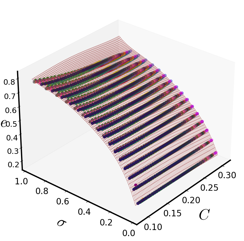
Universal relation for the star’s eccentricity \(e = \sqrt{1- \left(\frac{R_p}{R_e}\right)^2}\) (static NSs excluded)

x = 'C'; y = 'sigma'; z = 'eccentricity'; z_model = 'eccentricity_model'; x_power = 'C'; y_power = 'sigma';

Leave one out Cross validation

#cv_results = c_val_performace_results_for_k(df2,x='C',y='sigma',z='eccentricity')
#cv_results
#optim_pol_degree = int(cv_results[cv_results['d(%)'] == cv_results['d(%)'].min()]['k'].iloc[0])
#optim_pol_degree = 5

cv_results_e = pd.read_csv('LOOCV_results/e_LOOCV_results.txt')
cv_results_e

	MAE	Max_Error	MSE	d(%)	MAPE(%)	Explained_Variance	k
0	0.040421	0.156100	0.002398	61.983066	9.791475	1.0	1.0
1	0.013682	0.049544	0.000288	23.570241	3.323055	1.0	2.0
2	0.007252	0.037523	0.000080	11.369177	1.687115	1.0	3.0
3	0.005109	0.021952	0.000038	6.138886	1.082114	1.0	4.0
4	0.004652	0.019808	0.000033	4.576871	0.917538	1.0	5.0
5	0.004365	0.019091	0.000030	3.985076	0.836672	1.0	6.0
6	0.004357	0.018747	0.000029	3.896671	0.832603	1.0	7.0
7	0.004302	0.018830	0.000029	3.754733	0.822461	1.0	8.0

optim_pol_degree = 5

Linear regression on training data

df2[z_model], R_2_index, b_00, b_nm, power_comb_2, powers_2 = Regression_function(df2,x = x,y= y ,z=z, pol_degree=optim_pol_degree, 
                                        x_power = x_power,y_power = y_power)

\(R^2\) index

R_2_index

0.9987303980077309

Model’s coefficients

# model's intercept
b_00;
# model's coefficients
b_nm; 
# b_nm stored to data frame
coef=pd.DataFrame(b_nm,columns=["coef"])

def e_funct(C,sigma):
    results=0
    for i in range(0,len(powers_2)):
        results+=(coef["coef"][i]*C**(powers_2["C"][i])*sigma**(powers_2["sigma"][i]))
      
    return b_00 + results 

e_funct(C_s,sigma_s)

\[\displaystyle - 99.1731626257587 C^{5} + 68.055729822897 C^{4} \sigma + 137.191420601953 C^{4} + 12.9349885313228 C^{3} \sigma^{2} - 57.4743082972309 C^{3} \sigma - 67.7948794728821 C^{3} - 9.03315944594449 C^{2} \sigma^{3} + 8.0834606252312 C^{2} \sigma^{2} + 9.19713339469666 C^{2} \sigma + 14.9006458417103 C^{2} + 4.84885244516396 C \sigma^{4} - 6.44626099699597 C \sigma^{3} + 2.75499036217899 C \sigma^{2} - 1.33293692611052 C \sigma - 1.52533604289925 C + 4.714504734503 \sigma^{5} - 13.8547513636473 \sigma^{4} + 15.4712200610892 \sigma^{3} - 8.71280504897917 \sigma^{2} + 3.04229899830747 \sigma + 0.182560763719317\]

x2 = mesh_grid_funct(3000,df2,x_name = 'C', y_name = 'sigma')[0]
y2 = mesh_grid_funct(3000,df2, x_name = 'C', y_name = 'sigma')[1]

Z2 = e_funct(x2,y2)

def Surface_plot_funct_e(eos_data, x,y,z, xlabel,ylabel,zlabel, view2, n_col, border_axes, X,Y,Z, l_w):

    
    fig = plt.figure(figsize=(12, 8)) 
    labels_text_size = 25
    ax = fig.add_subplot(111, projection='3d')

    dot_size = 40
    font_size = 35
    label_pad = 25
    label_size = 25


    for i in range(0, len(eos_data)):
        ax.scatter3D(eos_data[i][x].to_numpy(),eos_data[i][y].to_numpy(),eos_data[i][z].to_numpy(),
                     s=dot_size, c=c_color[i], label = eos_labels[i])    

    
    ax.plot_wireframe(X, Y, Z, rstride=40, cstride=40,edgecolor='blue' ,color = 'maroon',
                      alpha=0.8, lw = l_w, antialiased=True)

    
    
    ax.view_init(30, view2)   
    ax.set_xlabel(xlabel, fontsize=font_size, labelpad=label_pad) 
    ax.set_ylabel(ylabel, fontsize=font_size, labelpad=label_pad) 
    ax.set_zlabel(zlabel, fontsize=font_size, labelpad=label_pad) 

    ax.zaxis.labelpad = 12 
    

    ax.xaxis.set_tick_params(labelsize=label_size-5)
    ax.yaxis.set_tick_params(labelsize=label_size-5)
    ax.zaxis.set_tick_params(labelsize=label_size-7)

    ax.zaxis.labelpad = 1
    for axis in [ax.xaxis, ax.yaxis, ax.zaxis]:
        axis.line.set_linewidth(3)
    
    ax.grid(False)

    
    plt.tight_layout()
    plt.show()   

Surface_plot_funct_e(eos_data2, x, y, z, xlabel=r'$C$',ylabel='$\sigma$',zlabel=r'$e$', 
                     view2=220, n_col=3, border_axes=8, X=x2,Y=y2,Z=Z2, l_w=0.5)

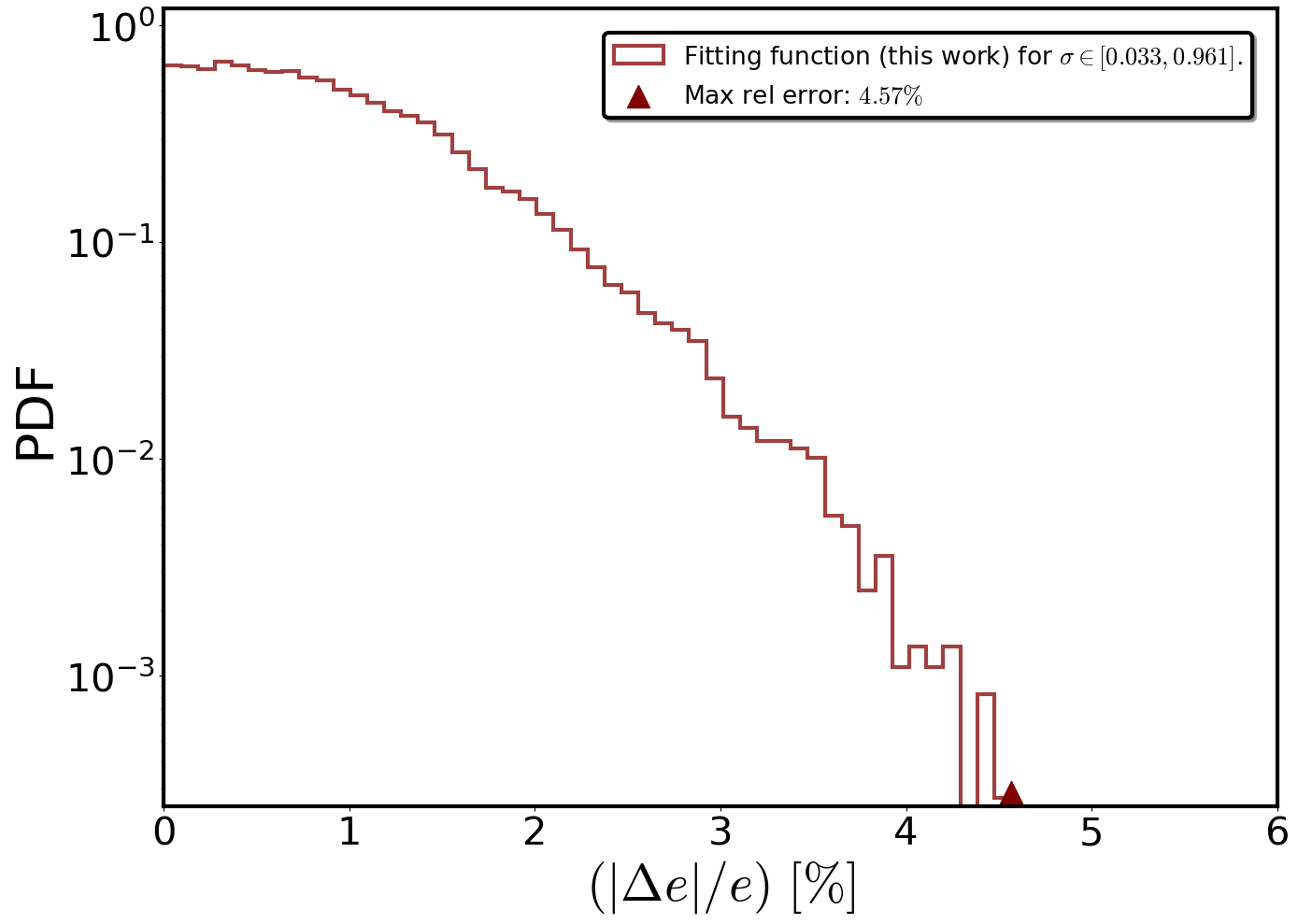
Fitting function’s percentage error distribution

fig,ax = plt.subplots(figsize=(14, 10),)
labels_text_size = 40
plt.xticks(fontsize=30) 
plt.yticks(fontsize=30)

xlabel = r'$(|\Delta e| /e) \ [\%]$'
ylabel = r'PDF'

plt.xlabel(xlabel,size=labels_text_size)
plt.ylabel(ylabel,size=labels_text_size)

bins = 50
alpha = 0.75

y_reg_model = (np.abs(100*(-df2[z] + df2[z_model])/df2[z])).hist(
    density=True, 
    bins=bins, 
    lw=3, 
    edgecolor='maroon', 
    zorder=1, 
    histtype='step', 
    alpha=alpha, 
    label=f"Fitting function (this work) for $ \sigma \in[{np.round(df2['sigma'].min(), 3)}, {np.round(df2['sigma'].max(), 3)}]$.", 
    color='maroon',
    #log = True
).autoscale(enable=True, axis='both', tight=True)


vertical_lines = [4.5660]  

plt.scatter(vertical_lines[0], 2.9e-4, color='maroon',  marker='^', s=300, zorder=2, label=r'Max rel error: $ 4.57 \%$')  

for axis in ['top','bottom','left','right']:
    ax.spines[axis].set_linewidth(3.)


plt.yscale('log')
plt.xlim(0,6)
plt.ylim(2.5e-4,1.2)

plt.grid(False)
leg = plt.legend(loc="upper right",ncol=1, borderaxespad=1, prop={'size': 19}, shadow=True, fontsize="large")    
leg.get_frame().set_linewidth(3.0)
leg.get_frame().set_edgecolor('black')

plt.tight_layout()
plt.show()

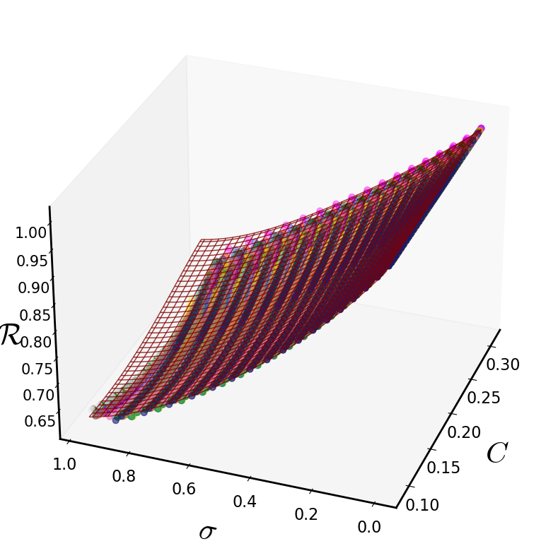
Universal relation for \(\mathcal{R} = R_p/R_{eq}\) (All NSs included)

x = 'C'; y = 'sigma'; z = 'Rpol/Req'; z_model = 'Rpol/Req_model'; x_power = 'C'; y_power = 'sigma'; #Rpol/Req

Leave one out Cross validation

#cv_results = c_val_performace_results_for_k(df,x='C',y='sigma',z='Rpol/Req')
#cv_results
#optim_pol_degree = int(cv_results[cv_results['d(%)'] == cv_results['d(%)'].min()]['k'].iloc[0])

cv_results_R = pd.read_csv('LOOCV_results/Rpol_Req_LOOCV_results.txt')
cv_results_R

	MAE	Max_Error	MSE	d(%)	MAPE(%)	Explained_Variance	k
0	0.011254	0.068301	0.000196	10.826695	1.401666	1.0	1.0
1	0.003819	0.027850	0.000025	4.414587	0.489926	1.0	2.0
2	0.003213	0.019550	0.000019	3.117947	0.421023	1.0	3.0
3	0.003112	0.018761	0.000019	2.801806	0.409053	1.0	4.0
4	0.003089	0.019980	0.000019	2.948913	0.405631	1.0	5.0
5	0.003067	0.020069	0.000018	2.962009	0.402397	1.0	6.0
6	0.003043	0.020626	0.000018	3.152602	0.398805	1.0	7.0
7	0.003014	0.020130	0.000018	3.076814	0.394644	1.0	8.0

optim_pol_degree = 4

LInear regression on training data

df[z_model], R_2_index, C_00, C_nm, pow_comb_3, powers_3 = Regression_function(df,x = x,y= y ,z=z, pol_degree=optim_pol_degree, 
                                        x_power = x_power,y_power = y_power)

\(R^2\) index

 R_2_index

0.9983153014546605

Model’s coefficients

# model's intercept
C_00;
# model's coefficients
C_nm;
# C_nm stored to data frame
coef=pd.DataFrame(C_nm,columns=["coef"])

def R_funct(C,sigma):
    results=0
    for i in range(0,len(powers_3)):
        results+=(coef["coef"][i]*C**(powers_3["C"][i])*sigma**(powers_3["sigma"][i]))
      
    return C_00 + results 

R_funct(C_s,sigma_s)

\[\displaystyle - 45.3015234274801 C^{4} - 7.52466249012259 C^{3} \sigma + 36.1318805958812 C^{3} - 2.50668582910242 C^{2} \sigma^{2} + 8.66838156199219 C^{2} \sigma - 10.4561101976216 C^{2} + 0.527775373801867 C \sigma^{3} - 0.226904263928412 C \sigma^{2} - 1.45892092679705 C \sigma + 1.29663161750561 C + 0.196118434593753 \sigma^{4} - 0.440968195037673 \sigma^{3} + 0.544639042230603 \sigma^{2} - 0.617710700567153 \sigma + 0.942328028476575\]

x3 = mesh_grid_funct(1500,df,x_name = 'C', y_name = 'sigma')[0]
y3 = mesh_grid_funct(1500,df, x_name = 'C', y_name = 'sigma')[1]

Z3 = R_funct(x3,y3)

def Surface_plot_funct_R(eos_data, x,y,z, xlabel,ylabel,zlabel, view2, n_col, border_axes, X,Y,Z, l_w):
    
    fig = plt.figure(figsize=(12, 8)) 
    labels_text_size = 25
    ax = fig.add_subplot(111, projection='3d')

    dot_size = 40
    font_size = 30
    label_pad = 20
    label_size = 20

    for i in range(0, len(eos_data)):
        ax.scatter3D(eos_data[i][x].to_numpy(),eos_data[i][y].to_numpy(),eos_data[i][z].to_numpy(),
                     s=dot_size, c=c_color[i]) 

    
    ax.plot_wireframe(X, Y, Z, rstride=40, cstride=40,edgecolor='blue' ,color = 'maroon',
                      alpha=0.8, zorder = 15, lw = l_w, antialiased=True)
    
    
    
    ax.view_init(30, view2)   
    ax.set_xlabel(xlabel, fontsize=font_size, labelpad=label_pad) 
    ax.set_ylabel(ylabel, fontsize=font_size, labelpad=label_pad) 
    ax.zaxis.set_rotate_label(False) 
    ax.set_zlabel(zlabel, fontsize=font_size, labelpad=label_pad, rotation=0) 

    
    ax.zaxis.labelpad = 6
    
    
    ax.xaxis.set_tick_params(labelsize=label_size-4)
    ax.yaxis.set_tick_params(labelsize=label_size-4)
    ax.zaxis.set_tick_params(labelsize=label_size-5)
    
    for axis in [ax.xaxis, ax.yaxis, ax.zaxis]:
        axis.line.set_linewidth(2)
    
    ax.grid(False)

    plt.tight_layout()
    plt.show()    
    

Surface_plot_funct_R(eos_data, x, y, z, xlabel=r'$C$',ylabel='$\sigma$',zlabel=r'$\mathcal{R}$', 
                     view2=200, n_col=1, border_axes=1, X=x3,Y=y3,Z=Z3, l_w=1.)

Absolute relative error distribution

fig,ax = plt.subplots(figsize=(14, 10),)
labels_text_size = 40
plt.xticks(fontsize=30) 
plt.yticks(fontsize=30)


xlabel = r'$(|\Delta \mathcal{R}| /\mathcal{R}) \ [\%]$'
ylabel = r'PDF'

plt.xlabel(xlabel,size=labels_text_size)
plt.ylabel(ylabel,size=labels_text_size)

bins = 50
alpha = 0.75

y_reg_model = abs(100*(-df[z]+df[z_model])/df[z]).hist(
    
    density = True,
    bins=bins,
    lw = 3,
    edgecolor ='maroon', 
    histtype='step', 
    alpha = alpha, 
    label = f"Fitting Function (this work) for $[0.000, {np.round(df['sigma'].max(), 3)}]$.", 
    color = 'maroon').autoscale(enable = True, axis = 'both', tight = True)


vertical_lines = [2.79] 
plt.scatter(vertical_lines[0], 2.9e-4, color='maroon',  marker='^', s=300, zorder=2, label=r'Max rel error: $ 2.79 \%$')  

y_reg_less_0_25 = abs(100*(-df[df['sigma']<=0.25][z]+df[df['sigma']<=0.25][z_model])/df[df['sigma']<=0.25][z]).hist(
    
    density = True,
    bins=bins,
    edgecolor ='coral',
    lw = 3,
    histtype='step', 
    zorder = 1, 
    alpha = alpha,
    label = f"Fitting Function (this work) for $\sigma \in[0.000, 0.250]$.",
    color = 'coral').autoscale(enable = True, axis = 'both', tight = True)


vertical_lines = [0.9581596145435877, None]  
plt.scatter(vertical_lines[0], 2.9e-4, color='coral',  marker='^', s=300, zorder=2, label=r'Max rel error: $ 0.96 \%$')  

plt.yscale('log')
plt.xscale('log')


plt.xlim(1e-1,20)
plt.ylim(2.5e-4,130)


for axis in ['top','bottom','left','right']:
    ax.spines[axis].set_linewidth(3.0)

plt.grid(False)
leg = plt.legend(loc="upper right",ncol=2, borderaxespad=1, prop={'size': 16}, shadow=True, fontsize="large")    
leg.get_frame().set_linewidth(3.0)
leg.get_frame().set_edgecolor('black')

plt.tight_layout()
plt.show()

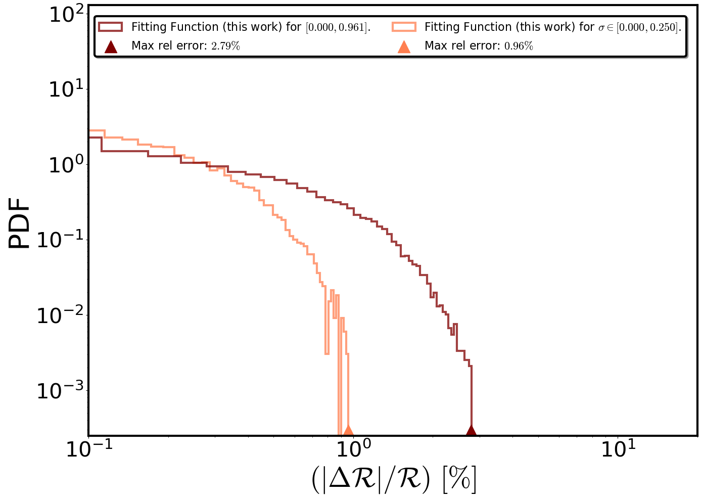
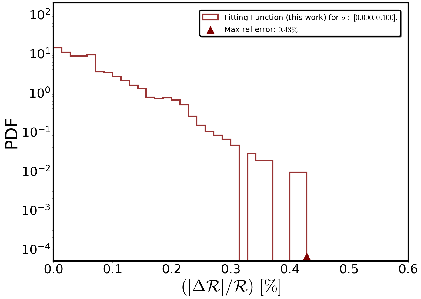
Slowly rotating case: Absolute relative error distribution

fig,ax = plt.subplots(figsize=(14, 10),)
labels_text_size = 40
plt.xticks(fontsize=30) 
plt.yticks(fontsize=30)


xlabel = r'$(|\Delta \mathcal{R}| /\mathcal{R}) \ [\%]$'
ylabel = f'PDF'

plt.xlabel(xlabel,size=labels_text_size)
plt.ylabel(ylabel,size=labels_text_size)

bins = 50
alpha = 0.8
y_reg_0_1_model = abs(100*(-df[df['sigma']<=0.1][z]+df[df['sigma']<=0.1][z_model])/df[df['sigma']<=0.1][z]).hist(
                    density = True,
                    bins=bins-20,
                    lw=3, 
                    edgecolor ='maroon', 
                    zorder = 1, 
                    histtype='step',
                    alpha = alpha,
                    label = f'Fitting Function (this work) for $\sigma \in[0.000, 0.100]$.', color = 'maroon').autoscale(enable = True, axis = 'both', tight = True)


vertical_lines_reg_0_1 = [0.42818322]  
plt.scatter(vertical_lines_reg_0_1[0], 0.65e-4, color='maroon',  marker='^', s=300, zorder=2, label=r'Max rel error: $ 0.43 \%$')  
plt.yscale('log')

plt.ylim(0.5e-4,200)
plt.xlim(0,0.6)


for axis in ['top','bottom','left','right']:
    ax.spines[axis].set_linewidth(3.0)

plt.grid(False)
leg = plt.legend(loc="upper right",ncol=1, borderaxespad=1, prop={'size': 18}, shadow=True, fontsize="large")   
leg.get_frame().set_linewidth(3.0)
leg.get_frame().set_edgecolor('black')
    
plt.tight_layout()
plt.show()

Nonrotating limit

fig,ax = plt.subplots(figsize=(14, 10),)  

labels_text_size = 50
plt.xticks(fontsize=30) 
plt.yticks(fontsize=30)

plt.xlabel(r'$C$',size=labels_text_size)
plt.ylabel(r'$ \left(\frac{|\Delta \mathcal{R}|}{\mathcal{R}}\right) \ [\%]$',size=labels_text_size)

plt.scatter(df_static['C'],100*abs((R_funct(df_static['C'],0))-df_static['Rpol/Req'])/df_static['Rpol/Req'], color = 'firebrick')  

for axis in ['top','bottom','left','right']:
    ax.spines[axis].set_linewidth(3.0)


plt.yscale('log')

plt.tight_layout()
plt.show()

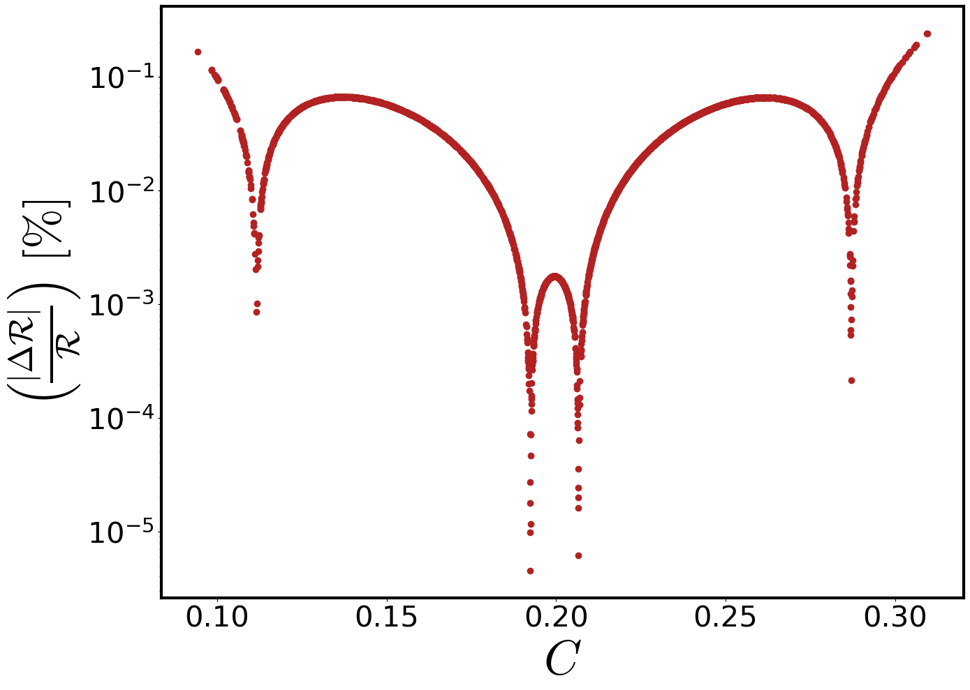
(100*abs((R_funct(df_static['C'],0))-df_static['Rpol/Req'])/df_static['Rpol/Req']).max()

0.24219577943114245

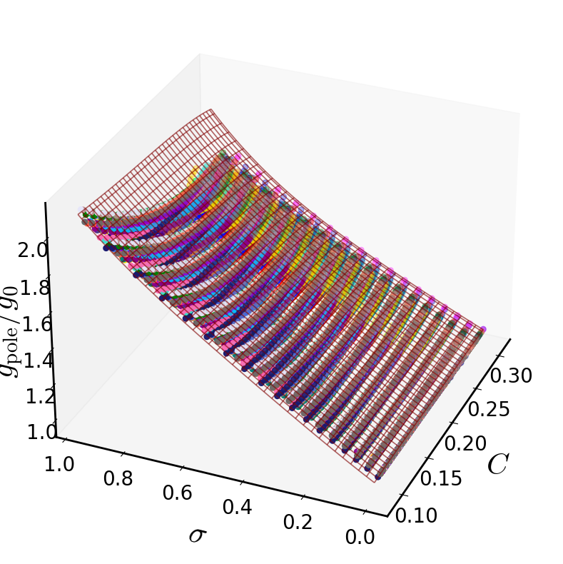
Universal relation for \(g_{pole}\)

x = 'C'; y = 'sigma'; z = 'g_pole_scaled' ; z_model = 'g_pole_scaled_model'; x_power = 'C'; y_power = 'sigma';

Leave one out Cross validation

#cv_results = c_val_performace_results_for_k(df,x=x,y=y,z=z)
#cv_results
#optim_pol_degree = int(cv_results[cv_results['d(%)'] == cv_results['d(%)'].min()]['k'].iloc[0])

cv_results_g_p = pd.read_csv('LOOCV_results/g_pole_LOOCV_results.txt')
cv_results_g_p 

	MAE	Max_Error	MSE	d(%)	MAPE(%)	Explained_Variance	k
0	0.015713	0.146115	0.000430	6.934889	1.176683	1.0	1.0
1	0.005539	0.078188	0.000072	4.101918	0.384596	1.0	2.0
2	0.004535	0.062011	0.000056	3.253231	0.303176	1.0	3.0
3	0.004320	0.053770	0.000052	3.073449	0.286016	1.0	4.0
4	0.004268	0.051413	0.000051	3.058724	0.282789	1.0	5.0
5	0.004222	0.053163	0.000050	2.967900	0.280160	1.0	6.0
6	0.004171	0.055593	0.000049	3.096514	0.277813	1.0	7.0
7	0.004090	0.057886	0.000047	3.224207	0.272419	1.0	8.0

optim_pol_degree = 4

Linear regression on training data

df[z_model], R_2_index, D_00, D_nm, pow_comb_4, powers_4 = Regression_function(df,x = x,y= y ,z=z, 
                                                  pol_degree=optim_pol_degree, x_power = x_power,
                                                  y_power = y_power)

\(R^2\) index

R_2_index

0.9991471134868862

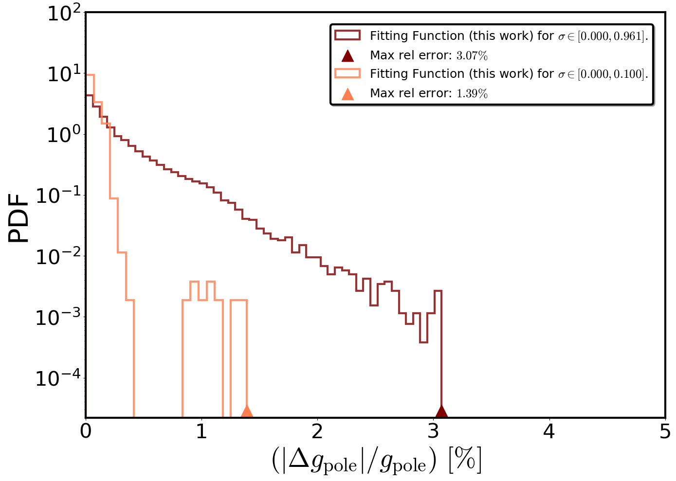
Fractional difference distribution

fig,ax = plt.subplots(figsize=(14, 10),)
labels_text_size = 40
plt.xticks(fontsize=30) 
plt.yticks(fontsize=30)

xlabel = r'$(|\Delta g_{\mathrm{pole}}| /g_{\mathrm{pole}}) \ [\%]$'
ylabel = 'PDF'

plt.xlabel(xlabel,size=labels_text_size)
plt.ylabel(ylabel,size=labels_text_size)

bins = 50
alpha = 0.8

y_reg_grav_model = abs(100*(-df[z]+df[z_model])/df[z]).hist(
                    density = True,
                    lw = 3,
                    bins=bins,
                    edgecolor ='maroon',
                    histtype='step',
                    zorder = 1, 
                    label = f"Fitting Function (this work) for $\sigma \in[0.000, {np.round(df['sigma'].max(), 3)}]$.", 
                    alpha = alpha,
                    color = 'maroon').autoscale(enable = True, axis = 'both', tight = True)


vertical_lines = [3.070871712452435]  
plt.scatter(vertical_lines[0], 2.9e-5, color='maroon',  marker='^', s=300, zorder=2, label=r'Max rel error: $ 3.07 \%$')  


y_reg_grav_model = abs(100*(-df[df['sigma']<=0.1][z]+df[df['sigma']<=0.1][z_model])/df[df['sigma']<=0.1][z]).hist(
                    density = True,
                    lw = 3,
                    bins=bins-30,
                    edgecolor ='coral',
                    histtype='step',
                    zorder = 1, 
                    label = r"Fitting Function (this work) for $\sigma \in[0.000, 0.100]$.", 
                    alpha = alpha,
                    color = 'coral').autoscale(enable = True, axis = 'both', tight = True)


vertical_lines = [1.391]  
plt.scatter(vertical_lines[0], 2.9e-5, color='coral',  marker='^', s=300, zorder=2, label=r'Max rel error: $ 1.39 \%$')  


plt.yscale('log')
plt.xlim(0,5)

plt.ylim(2.2e-5,100)

for axis in ['top','bottom','left','right']:
    ax.spines[axis].set_linewidth(3.0)

plt.grid(False)
leg = plt.legend(loc="upper right",ncol=1, borderaxespad=1, prop={'size': 18}, shadow=True, fontsize="large")    
leg.get_frame().set_linewidth(3.0)
leg.get_frame().set_edgecolor('black')
    
plt.tight_layout()
plt.show()

Model’s coefficients

# model's intercept
D_00; 
# model's coefficients
D_nm;
# D_nm stored to data frame
coef=pd.DataFrame(D_nm,columns=["coef"])

def g_pole_funct(C,sigma):
    results=0
    for i in range(0,len(powers_4)):
        results+=(coef["coef"][i]*C**(powers_4["C"][i])*sigma**(powers_4["sigma"][i]))
      
    return D_00 + results 

g_pole_funct(C_s,sigma_s)

\[\displaystyle - 62.8045467352433 C^{4} - 23.257769499827 C^{3} \sigma + 52.0686732207975 C^{3} + 1.11602879356068 C^{2} \sigma^{2} + 11.9714816462283 C^{2} \sigma - 15.6899254468898 C^{2} + 1.4660608155789 C \sigma^{3} - 1.46935053803782 C \sigma^{2} - 2.79057152330362 C \sigma + 2.0186963881549 C + 0.488086658631061 \sigma^{4} - 0.800025443187702 \sigma^{3} + 0.553202313363455 \sigma^{2} + 1.08421869564886 \sigma + 0.908110925704063\]

x4 = mesh_grid_funct(1500,df,x_name = 'C', y_name = 'sigma')[0]
y4 = mesh_grid_funct(1500,df, x_name = 'C', y_name = 'sigma')[1]

Z4 = g_pole_funct(x4,y4)

def Surface_plot_funct_gp(eos_data, x,y,z, xlabel,ylabel,zlabel, view2, n_col, border_axes, X,Y,Z, l_w):
    
    fig = plt.figure(figsize=(12, 8)) 
    labels_text_size = 28
    ax = fig.add_subplot(111, projection='3d')

    dot_size = 30
    font_size = 30
    label_pad = 20
    label_size = 20

    for i in range(0, len(eos_data)):
        ax.scatter3D(eos_data[i][x].to_numpy(),eos_data[i][y].to_numpy(),eos_data[i][z].to_numpy(),
                     s=dot_size, c=c_color[i])  #, label = eos_labels[i]  

    
    ax.plot_wireframe(X, Y, Z, rstride=40, cstride=40,edgecolor='blue' ,color = 'maroon',
                      alpha=0.6, zorder = 15, lw = l_w, antialiased=True)
    
    
    
    ax.view_init(30, view2)   
    ax.set_xlabel(xlabel, fontsize=font_size, labelpad=label_pad) 
    ax.set_ylabel(ylabel, fontsize=font_size, labelpad=label_pad) 
    
    ax.zaxis.set_rotate_label(False) 
    ax.set_zlabel(zlabel, fontsize=font_size,labelpad=label_pad,rotation = 90)
    ax.zaxis.set_tick_params(pad=0)
    ax.zaxis.labelpad = 5
    

    ax.zaxis._axinfo['label']['space_factor'] = 10.0
 
    ax.xaxis.set_tick_params(labelsize=label_size)
    ax.yaxis.set_tick_params(labelsize=label_size)
    ax.zaxis.set_tick_params(labelsize=label_size)
    
    for axis in [ax.xaxis, ax.yaxis, ax.zaxis]:
        axis.line.set_linewidth(2)
    
    ax.grid(False)
    
    plt.tight_layout()
    plt.show()
    

Surface_plot_funct_gp(eos_data, x, y, z, xlabel=r'$C$',ylabel='$\sigma$',zlabel=r'$g_{\mathrm{pole}}/g_0$', 
                     view2=203, n_col=3, border_axes=8, X=x4,Y=y4,Z=Z4, l_w=1.2)

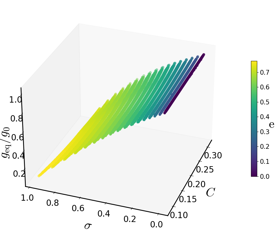
Universal relation for \(g_{eq}\)

x = 'C'; y = 'sigma'; w = 'eccentricity' ;z = 'g_eq_scaled' ; z_model = 'g_eq_scaled_model';

Leave one out Cross validation

#cv_results = c_val_performace_results_for_k_2(df,x=x,y=y,w=w,z=z)
#cv_results
#optim_pol_degree = int(cv_results[cv_results['d(%)'] == cv_results['d(%)'].min()]['k'].iloc[0])

cv_results_g_eq = pd.read_csv('LOOCV_results/g_eq_LOOCV_results')
cv_results_g_eq

	MAE	Max_Error	MSE	d(%)	MAPE(%)	Explained_Variance	k
0	0.012457	0.090990	2.345235e-04	60.239597	2.356113	1.0	1.0
1	0.003238	0.028102	1.992911e-05	40.535751	0.643018	1.0	2.0
2	0.000760	0.012911	1.232216e-06	4.337101	0.169832	1.0	3.0
3	0.000646	0.012945	1.010815e-06	3.838275	0.147062	1.0	4.0
4	0.000597	0.013014	9.265978e-07	3.448856	0.137110	1.0	5.0
5	0.000582	0.013116	9.029801e-07	2.856619	0.134236	1.0	6.0
6	0.000573	0.013054	8.834424e-07	2.769864	0.131815	1.0	7.0
7	0.000560	0.013089	8.552114e-07	2.777353	0.129038	1.0	8.0

optim_pol_degree = 3

Linear regression on training data

df[z_model], R_2_index, E_00, E_nm, pow_comb_5, powers_5 = Regression_function_2(df,x = x,y = y,w = w ,z = z, pol_degree=optim_pol_degree,
                                              x_power = x,y_power=y,w_power=w)

\(R^2\) index

R_2_index

0.9999763625907374

Model’s coefficients

# model's intercept
E_00;
# model's coefficients
E_nm;
# a_nm stored to data frame
coef=pd.DataFrame(E_nm,columns=["coef"])

E_nm

array([ 0.        ,  0.06866332, -1.69175782, -0.02976716, -0.28467956,
        2.33122575,  0.14131776,  0.53280091, -0.75836694,  0.83218179,
        0.33807042,  1.20592156,  0.12888786, -4.03577574,  2.63090429,
       -2.03273805, -0.22100945,  0.36927603,  0.23073066,  0.28904095])

def g_eq_funct(C,sigma,e):
    results=0
    for i in range(0,len(powers_5)):
        results+=(coef["coef"][i]*C**(powers_5["C"][i])*sigma**(powers_5["sigma"][i])*e**(powers_5["eccentricity"][i]))
      
    return E_00 + results 

g_eq_funct(C_s,sigma_s, e_s)

\[\displaystyle 0.338070419688191 C^{3} + 1.20592155663032 C^{2} \sigma + 0.128887857187797 C^{2} e - 0.284679560623361 C^{2} - 4.0357757427521 C \sigma^{2} + 2.63090429234693 C \sigma e + 2.33122575049243 C \sigma - 2.03273805025505 C e^{2} + 0.141317760072622 C e + 0.0686633222621077 C - 0.221009453432658 \sigma^{3} + 0.369276028155004 \sigma^{2} e + 0.532800911941009 \sigma^{2} + 0.23073065963261 \sigma e^{2} - 0.758366940518667 \sigma e - 1.69175782343621 \sigma + 0.289040948522035 e^{3} + 0.832181789667688 e^{2} - 0.0297671570402134 e + 0.995124108230518\]

x5 = mesh_grid_funct_2(100,df,x_name = 'C', y_name = 'sigma', w_name = 'eccentricity')[0]
y5 = mesh_grid_funct_2(100,df, x_name = 'C', y_name = 'sigma', w_name = 'eccentricity')[1]
w5 = mesh_grid_funct_2(100,df, x_name = 'C', y_name = 'sigma', w_name = 'eccentricity')[2]

Z5 = g_eq_funct(x5,y5,w5)

def Surface_plot_funct_geq(eos_data, x,y,w, z, xlabel,ylabel,wlabel,zlabel, view2, n_col,
                         border_axes, X,Y,W, Z, l_w):
    
    fig = plt.figure(figsize=(12, 8)) 
    labels_text_size = 28
    ax = fig.add_subplot(111, projection='3d')

    dot_size = 30
    font_size = 30
    label_pad = 20
    label_size = 20    

    for i in range(0, len(eos_data)):
        scatter = ax.scatter(eos_data[i][x].to_numpy(),eos_data[i][y].to_numpy(),eos_data[i][z].to_numpy(),
                   c = eos_data[i][w].to_numpy(), s = dot_size, cmap='viridis', marker='o')    
    
    
    # Add colorbar
    cbar = plt.colorbar(scatter,  shrink=0.5)
    cbar.set_label(wlabel, fontsize=font_size,rotation=0)
    cbar.ax.tick_params(labelsize=15)
        
    ax.view_init(30, view2)   
    ax.set_xlabel(xlabel, fontsize=font_size,labelpad=label_pad) 
    ax.set_ylabel(ylabel, fontsize=font_size,labelpad=label_pad) 
    
    ax.zaxis.set_rotate_label(False) 
    ax.set_zlabel(zlabel, fontsize=font_size,labelpad=label_pad,rotation = 90)

    ax.zaxis._axinfo['label']['space_factor'] = -30.0
    
    ax.zaxis.set_tick_params(pad=0.)
    ax.zaxis.labelpad = 5#0.4 
    
    ax.xaxis.set_tick_params(labelsize=label_size)
    ax.yaxis.set_tick_params(labelsize=label_size)
    ax.zaxis.set_tick_params(labelsize=label_size)
    
    for axis in [ax.xaxis, ax.yaxis, ax.zaxis]:
        axis.line.set_linewidth(2)
    
    ax.grid(False)
    
    plt.tight_layout()    
    plt.show()

Surface_plot_funct_geq(eos_data, x,y,w,z, xlabel=r'$C$',ylabel='$\sigma$',
                     wlabel = r'$\mathrm{e}$',zlabel=r'$g_{\mathrm{eq}}/g_0$', 
                     view2=200, n_col=3, border_axes=8, X=x5,Y=y5,W = w5,Z=Z5, l_w=1.5)

Absolute relative error distribution

fig,ax = plt.subplots(figsize=(14, 10),)
labels_text_size = 40
plt.xticks(fontsize=30) 
plt.yticks(fontsize=30)

xlabel = r'$(|\Delta g_{\mathrm{eq}}| /g_{\mathrm{eq}}) \ [\%]$'
ylabel = 'PDF'



plt.xlabel(xlabel,size=labels_text_size)
plt.ylabel(ylabel,size=labels_text_size)

bins = 45
alpha = 0.8


y_reg_grav_model = abs(100*(-df[z]+df[z_model])/df[z]).hist(
    density = True,
    bins=bins-20,
    lw = 3,
    edgecolor ='maroon', 
    histtype='step',
    zorder = 1, 
    alpha = alpha,
    label = f"Fitting Function (this work) for $\sigma \in [0.000, {np.round(df2['sigma'].max(), 3)}]$.", color = 'maroon').autoscale(enable = True, axis = 'both', tight = True)


vertical_lines = [4.264130569493755, None]  
plt.scatter(vertical_lines[0], 0.65e-5, color='maroon', marker='^', s=300, zorder=2, label=r'Max rel error: $4.26\%$')  


y_reg_grav_model = abs(100*(-df[df['sigma']<=0.1][z]+df[df['sigma']<=0.1][z_model])/df[df['sigma']<=0.1][z]).hist(
    density = True,
    bins=bins-30,
    lw = 3,
    edgecolor ='coral', 
    histtype='step',
    zorder = 1, 
    alpha = alpha,
    label = f"Fitting Function (this work) for $\sigma \in [0.000, 0.100]$.", 
   color = 'coral').autoscale(enable = True, axis = 'both', tight = True)


vertical_lines = [1.307, None] 
plt.scatter(vertical_lines[0], 0.65e-5, color='coral', marker='^', s=300, zorder=2, label=r'Max rel error: $1.31\%$')  

plt.yscale('log')
plt.xscale('log')


plt.ylim(0.5e-5,1000)
plt.xlim(0.5e-1,120)

for axis in ['top','bottom','left','right']:
    ax.spines[axis].set_linewidth(3.0)

plt.grid(False)
leg = plt.legend(loc="upper right",ncol=1, borderaxespad=1, prop={'size': 17}, shadow=True, fontsize="large")    
leg.get_frame().set_linewidth(3.0)
leg.get_frame().set_edgecolor('black')
    
plt.tight_layout()
plt.show()

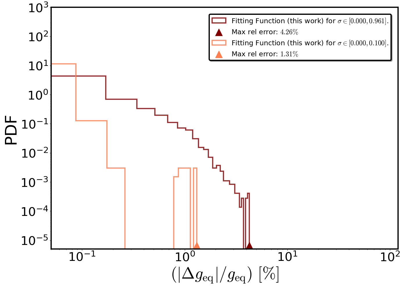
abs(100*(-df[z]+df[z_model])/df[z]).max()

4.264130569493755

abs(100*(-df[df['sigma']<=0.1][z]+df[df['sigma']<=0.1][z_model])/df[df['sigma']<=0.1][z]).max()

1.3072154897475385

EoS insensitive relation for \((d\log R/d \theta) max\)

x = 'C'; y = 'sigma'; w = 'Rpol/Req' ;z = 'dlogR_dtheta_max' ; z_model = 'dlogR_dtheta_max_model';

Leave one out Cross validation

#cv_results = c_val_performace_results_for_k_2(df2,x=x,y=y,w=w,z=z)
#cv_results
#optim_pol_degree = int(cv_results[cv_results['d(%)'] == cv_results['d(%)'].min()]['k'].iloc[0])

cv_results_dLogR = pd.read_csv('LOOCV_results/dLogR_dtheta_LOOCV_results.txt')
cv_results_dLogR

	MAE	Max_Error	MSE	d(%)	MAPE(%)	Explained_Variance	k
0	0.003774	0.026318	2.375680e-05	79.081525	4.046781	1.0	1.0
1	0.000669	0.021541	1.258866e-06	5.234422	0.395973	1.0	2.0
2	0.000497	0.007817	7.828603e-07	3.227351	0.231198	1.0	3.0
3	0.000438	0.007156	6.900567e-07	5.798164	0.182552	1.0	4.0
4	0.000416	0.006877	6.532774e-07	2.612371	0.169510	1.0	5.0
5	0.000403	0.006840	6.320654e-07	3.912433	0.159825	1.0	6.0
6	0.000395	0.006831	6.143983e-07	2.627716	0.157560	1.0	7.0
7	0.000382	0.006846	5.988247e-07	3.535615	0.144146	1.0	8.0

optim_pol_degree = 3

Linear regression on training data

df2[z_model], R_2_index, F_00, F_nm, pow_comb_6, powers_6 = Regression_function_2(df2,x = x,y= y, w = w ,z = z, 
                           pol_degree=optim_pol_degree, x_power = x,y_power=y, w_power = w)

\(R^2\) index

R_2_index

0.9999491798375334

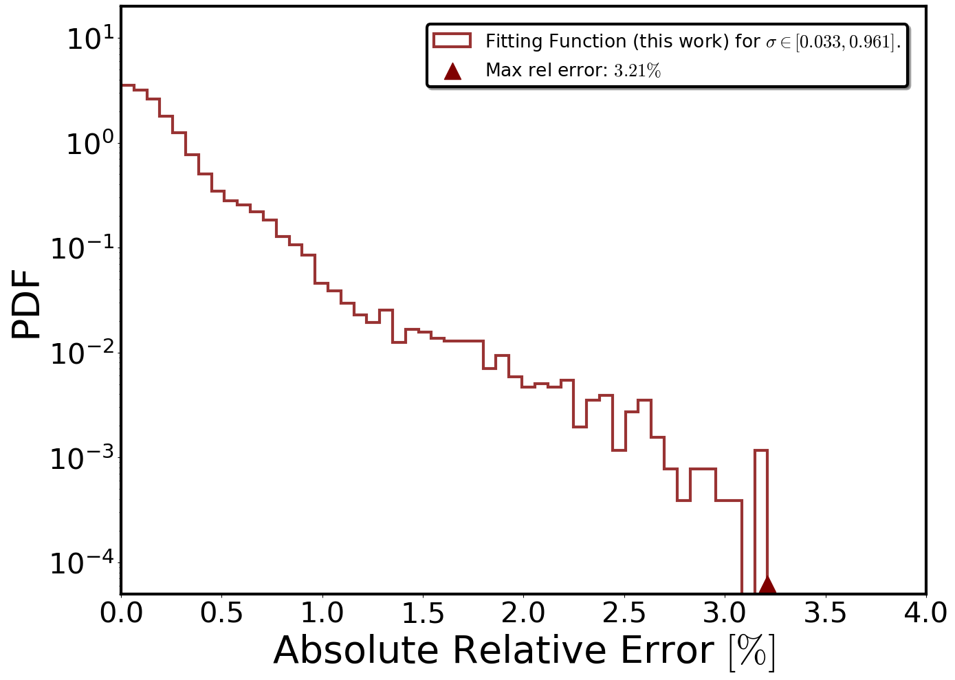
Absolute relative error distribution

fig,ax = plt.subplots(figsize=(14, 10),)
labels_text_size = 40
plt.xticks(fontsize=30) 
plt.yticks(fontsize=30)


xlabel = r'Absolute Relative Error$\ [\%]$'
ylabel = r'PDF'


plt.xlabel(xlabel,size=labels_text_size)
plt.ylabel(ylabel,size=labels_text_size)

bins = 50
alpha = 0.8

log_reg_model = abs(100*(-df2[z]+df2[z_model])/df2[z]).hist(
    density = True,
    lw = 3,
    bins=bins,
    edgecolor ='maroon',
    histtype='step',
    zorder = 1,
    alpha = alpha, 
    label = f"Fitting Function (this work) for $ \sigma \in[{np.round(df2['sigma'].min(), 3)}, {np.round(df2['sigma'].max(), 3)}]$.",
    color = 'maroon').autoscale(enable = True, axis = 'both', tight = True)

vertical_lines = [3.2128461268526847] 
plt.scatter(vertical_lines[0], 0.625e-4, color='maroon',  marker='^', s=300, zorder=2, label=r'Max rel error: $ 3.21 \%$')  

plt.yscale('log')

plt.ylim(0.5e-4,20)

plt.xlim(0,4)

for axis in ['top','bottom','left','right']:
    ax.spines[axis].set_linewidth(3.0)

plt.grid(False)
leg = plt.legend(loc="upper right",ncol=1, borderaxespad=1, prop={'size': 19}, shadow=True, fontsize="large")    
leg.get_frame().set_linewidth(3.0)
leg.get_frame().set_edgecolor('black')
    
plt.tight_layout()
plt.show()

Model’s coefficients

# model's intercept
F_00;
# model's coefficients
F_nm; 
# F_nm stored to data frame
coef=pd.DataFrame(F_nm,columns=["coef"])

def dLogR_dtheta_max_funct(C,sigma,R_s):
    results=0
    for i in range(0,len(powers_6)):
        results+=(coef["coef"][i]*C**(powers_6[x][i])*sigma**(powers_6[y][i])*R_s**(powers_6[w][i]))
      
    return F_00 + results 

dLogR_dtheta_max_funct(C_s,sigma_s, R_s)

\[\displaystyle - 0.403276601294769 C^{3} + 2.57434191156734 C^{2} \mathcal{R} + 0.66151909779781 C^{2} \sigma - 2.23108454812405 C^{2} - 45.0567823427942 C \mathcal{R}^{2} - 39.6796750694061 C \mathcal{R} \sigma + 87.0956609309219 C \mathcal{R} - 8.6762573974298 C \sigma^{2} + 38.4663786236091 C \sigma - 42.1349805655765 C + 53.9663039266245 \mathcal{R}^{3} + 72.1353182129612 \mathcal{R}^{2} \sigma - 146.85852284865 \mathcal{R}^{2} + 30.4880078789053 \mathcal{R} \sigma^{2} - 130.455828718701 \mathcal{R} \sigma + 131.341936932986 \mathcal{R} + 4.07991541887699 \sigma^{3} - 27.2418077134931 \sigma^{2} + 58.559061635722 \sigma - 38.441438473346\]

x6 = mesh_grid_funct_2(100,df2,x_name = x, y_name = y, w_name = w)[0]
y6 = mesh_grid_funct_2(100,df2, x_name = x, y_name = y, w_name = w)[1]
w6 = mesh_grid_funct_2(100,df2, x_name = x, y_name = y, w_name = w)[2]

Z6 = dLogR_dtheta_max_funct(x6,y6,w6)

def Surface_plot_funct_dlog(eos_data, x,y,w, z, xlabel,ylabel,wlabel,zlabel, view2, n_col,
                         border_axes, X,Y,W, Z, l_w):
    
    fig = plt.figure(figsize=(12, 8)) 
    labels_text_size = 24
    ax = fig.add_subplot(111, projection='3d')

    dot_size = 28
    font_size = 27
    label_pad = 20
    label_size = 20    
   
    for i in range(0, len(eos_data)):
        scatter = ax.scatter(eos_data[i][x].to_numpy(),eos_data[i][y].to_numpy(),eos_data[i][z].to_numpy(),
                   c = eos_data[i][w].to_numpy(), s = dot_size, cmap='viridis', marker='o')    
        
    cbar = plt.colorbar(scatter,  shrink=0.5)
    cbar.set_label(wlabel, fontsize=font_size, rotation=0)
    cbar.ax.tick_params(labelsize=15)
    
    
    ax.view_init(30, view2)   
    ax.set_xlabel(xlabel, fontsize=font_size,labelpad=label_pad) 
    ax.set_ylabel(ylabel, fontsize=font_size,labelpad=label_pad) 
    
    ax.zaxis.set_rotate_label(False) 
    ax.set_zlabel(zlabel, fontsize=font_size,labelpad=label_pad,rotation = 90) 
    ax.yaxis._axinfo['label']['space_factor'] = 3.0   

    ax.zaxis.set_tick_params(pad=0.)
    ax.zaxis.labelpad = 5
    
    ax.xaxis.set_tick_params(labelsize=label_size)
    ax.yaxis.set_tick_params(labelsize=label_size)
    ax.zaxis.set_tick_params(labelsize=label_size)
    
    for axis in [ax.xaxis, ax.yaxis, ax.zaxis]:
        axis.line.set_linewidth(2)
    
    ax.grid(False)
    
    plt.tight_layout()    
    plt.show()    

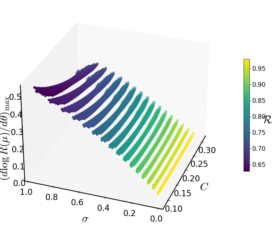
Surface_plot_funct_dlog(eos_data2, x,y,w,z, xlabel=r'$C$',ylabel='$\sigma$',
                     wlabel = r'$\mathcal{R}$',zlabel=r'$\left(d\log R(\mu)/ d\theta \right)_{\mathrm{max}}$', 
                     view2=200, n_col=3, border_axes=8, X=x6,Y=y6,W = w6,Z=Z6, l_w=1.5) #219