Logarithmic-Derivative Regressor Demo

Essential Libraries

import numpy as np
import pandas as pd
import matplotlib.pyplot as plt
from matplotlib.ticker import ScalarFormatter
from matplotlib.ticker import FuncFormatter
from matplotlib.tri import Triangulation, LinearTriInterpolator
import ipywidgets as widgets
from ipywidgets import interactive, FloatSlider
from IPython.display import display

from sklearn.metrics import explained_variance_score, max_error, mean_absolute_error
from sklearn.metrics import mean_squared_error, r2_score, mean_absolute_percentage_error

import UR_utils
from UR_utils import *

import torch
import torch.nn as nn
import torch.optim as optim
from torch.utils.data import DataLoader, TensorDataset
from DNN import Regressor

import os
import re
import time
from zipfile import ZipFile

from scipy import special
from scipy.interpolate import griddata

from matplotlib import rc
rc('mathtext', fontset='cm')

Global variables

device = torch.device('cuda:0' if torch.cuda.is_available() else 'cpu')

if torch.cuda.is_available():
    torch.cuda.set_device(device)

selected_columns = ['cos(theta)', 'R_surf', 'dlogR_dtheta', 'g_surf', 'Rpole_num', 'Req_num', 
                    'Rpol/Req', 'ellipticity', 'eccentricity', 'rho_c', 'r_ratio', 'M', 'M(km)',
                    'Req', 'C', 'K', 'g_0(km^(-1))', 'Ibar', 'f(Hz)', 'f_tilde', 'Jgeom(km^2)',
                    'x', 'sigma', 'T/W', 'Mxf_tilde', 'Rxf_tilde', 'Qbar', 'S3bar', 'EoS']

selected_features = ['cos(theta)', 'C', 'sigma', 'Rpol/Req']

abs_mu_min, abs_mu_max = 0., 1. 
C_min, C_max = 0.0876346858172578, 0.3094541325480277
sigma_min, sigma_max = 0., 0.9612274013913829
eccentricity_min, eccentricity_max = 0., 0.7797886226038347
Rpol_Req_min, Rpol_Req_max = 0.6260428931452016, 1.0

min_values = np.array([abs_mu_min, C_min, sigma_min, Rpol_Req_min])
max_values = np.array([abs_mu_max, C_max, sigma_max, Rpol_Req_max])

feature_scaler = lambda data: (data - min_values) / (max_values - min_values)

N_MU = 521

Read Star Data

def read_zip(file_name, spin, test_percentage=0.2):
    # random seed for 'freezing' randomness
    SEED = 42
    rng = np.random.default_rng(SEED)
    
    # specifying the zip file name
    columns_names = ['cos(theta)', 'R_surf', 'dlogR_dtheta', 'g_surf', 'Rpole_num', 'Req_num', 'Rpol/Req',
                    'ellipticity', 'eccentricity', 'P_c', 'rho_c', 'r_ratio', 'r_e', 'M', 'M(km)',
                    'Req', 'C', 'K', 'g_0(km^(-1))', 'I(kgkm^2)', 'I(km^3)', 'Ibar', 'Z_p', 'Z_b',
                    'Z_f', 'Ω(Hz)', 'f(Hz)', 'f_tilde', 'Jgeom(km^2)', 'x', 'sigma', 'T/W',
                    'Mxf_tilde', 'Rxf_tilde', 'conv_rad', 'conv_plus', 'conv_minus', 'h_plus',
                    'h_minus', 'r_plus', 'r_minus', 'Q(km^3)', 'Qbar', 'S3(km^4)', 'S3bar', 'M4_geom',
                    'M4_asy^GH_geom', 'M4_asy_geom', 'M4_geom_2points', 'M4_geom_3points',
                    'M4_geom_4points', 'S5_geom', 'S5_asy_geom', 'EoS']
    
    minmax_scale = lambda dR_dtheta, dR_dtheta_min, dR_dtheta_max: (dR_dtheta - dR_dtheta_min) / (dR_dtheta_max - dR_dtheta_min)

    df_train, df_test = pd.DataFrame(), pd.DataFrame()
    # opening the zip file in READ mode
    with ZipFile(file_name, 'r') as zip:
        # Pop the folder from the list of stars
        zip.infolist().pop(0)
        
        star_train, star_test = list(), list()
        n_stars = len(zip.infolist())
        n_test_stars = int(n_stars * test_percentage)
        test_indexes = rng.choice(n_stars, n_test_stars, replace=False)
        
        for index, star in enumerate(zip.infolist()):
            star = zip.extract(star)
            df_star = pd.read_csv(star, sep=' ', names=columns_names, skiprows=1)
            
            # Keep stars that only with r_ratio >= 0.6
            if df_star['r_ratio'].iloc[0] < 0.6: continue
            repeat_values = df_star.iloc[0].values
            df_star.iloc[1:, 4:] = repeat_values[4:]
            
            # Select only this columns to save memory
            df_star = df_star[selected_columns] 
            
            # Output normalization
            if np.all(df_star[spin] == 0.0):
                # Avoid zero division to static case
                df_star['dlogR_dtheta_scaled'] = 0.0
            else:
                # Min max scaling at star level
                df_star['dlogR_dtheta_scaled'] = minmax_scale(df_star['dlogR_dtheta'], 0.0, df_star['dlogR_dtheta'].max())
                                    
            if index in test_indexes:
                star_test.append(df_star)
            else:
                star_train.append(df_star)
                
        # Concat the dataframes to train and test
        if star_train: df_train = pd.concat(star_train, ignore_index=True)
        if star_test: df_test = pd.concat(star_test, ignore_index=True)
        
    return df_train, df_test

def load_stars(df, batch_size=4096, shuffle=True):
    df_target = df['dlogR_dtheta_scaled']
    
    np_features = df[selected_features].to_numpy()    
    np_targets = df_target.to_numpy()
    np_targets = np.reshape(np_targets, (np_targets.shape[0], 1))
    
    tr_features = torch.Tensor(feature_scaler(np_features))
    input_dimension = tr_features.shape[1]
    
    tr_targets = torch.Tensor(np_targets)
    final_dataset = TensorDataset(tr_features, tr_targets)

    # pin_memory=True, num_workers >= 1 if data is not already on device and model is training
    dataloader = DataLoader(final_dataset, batch_size=batch_size, shuffle=shuffle, num_workers=1, pin_memory=True)

    return dataloader, input_dimension, np_features, np_targets

Evaluation: statistical evaluation measures

Evaluation of the Logarithmic derivative ANN model performance to the whole NSs Dataset test set

df_eval_dataset = pd.read_csv('./Experimental Results/Derivative/dataset_measures.csv')
df_eval_dataset
#df_eval_dataset.to_latex(index = False, escape = False)

	explained_variance	max_error	mean_absolute_error	mean_squared_error	r2_score	mean_absolute_percentage_error	eval_eos_type	eval_eos_name
0	0.999976	0.00836	0.000266	3.186803e-07	0.999976	23264224.0	NaN	NaN

Evaluation of the Regression ANN model to the whole NS’s data (per EOS level) on the test set

df_eval_eos = pd.read_csv('./Experimental Results/Derivative/EOS_measures.csv')
df_eval_eos = df_eval_eos.sort_values(by = ['eval_eos_type', 'eval_eos_name'])
df_eval_eos.reset_index(drop = True, inplace = True)
df_eval_eos
#df_eval_eos.to_latex(index = False, escape = False)

	explained_variance	max_error	mean_absolute_error	mean_squared_error	r2_score	mean_absolute_percentage_error	eval_eos_type	eval_eos_name
0	0.999992	0.002905	0.000172	9.455648e-08	0.999992	46598380.0	Hadronic	BL_2018
1	0.999986	0.003635	0.000203	1.827745e-07	0.999986	22160074.0	Hadronic	BSK22
2	0.999986	0.004378	0.000210	1.922628e-07	0.999986	20966680.0	Hadronic	BSK24
3	0.999975	0.004886	0.000298	3.433152e-07	0.999974	18877362.0	Hadronic	BSK25
4	0.999983	0.005017	0.000219	1.993735e-07	0.999982	15456175.0	Hadronic	BSK26
...	...	...	...	...	...	...	...	...
65	0.999977	0.004800	0.000297	3.371826e-07	0.999975	18291932.0	Hyperonic	DS(CMF)-3
66	0.999991	0.002656	0.000179	1.142386e-07	0.999991	12745778.0	Hyperonic	DS(CMF)-5
67	0.999992	0.003068	0.000170	9.824574e-08	0.999992	12089122.0	Hyperonic	DS(CMF)-7
68	0.999990	0.004050	0.000199	1.471445e-07	0.999990	13917331.0	Hyperonic	GM1 Y5
69	0.999989	0.003393	0.000212	1.554367e-07	0.999989	14820256.0	Hyperonic	GM1 Y6

70 rows × 8 columns

Evaluation measures for the trained ANN model to the star level [NSs at test dataset]

#note: follow the ./Experimental Results/Derivative/ path and unzip the error_star_level.zip file
df = pd.read_csv('./Experimental Results/Derivative/error_star_level.csv')

df

	Unnamed: 0	residual	star_id	mu	Req	C	sigma	eccentricity	Rpol/Req	dlogR_dtheta_scaled	eval_eos_type	eval_eos_name
0	0	1.334784e-06	0	0.000000	16.1732	0.207095	0.735137	7.301570e-01	0.683279	0.000000	Hyperonic	DS(CMF)-5
1	1	-3.184690e-04	0	0.001923	16.1732	0.207095	0.735137	7.301570e-01	0.683279	0.012673	Hyperonic	DS(CMF)-5
2	2	-7.212907e-05	0	0.003846	16.1732	0.207095	0.735137	7.301570e-01	0.683279	0.024923	Hyperonic	DS(CMF)-5
3	3	-2.482794e-04	0	0.005769	16.1732	0.207095	0.735137	7.301570e-01	0.683279	0.037454	Hyperonic	DS(CMF)-5
4	4	3.697407e-04	0	0.007692	16.1732	0.207095	0.735137	7.301570e-01	0.683279	0.049983	Hyperonic	DS(CMF)-5
...	...	...	...	...	...	...	...	...	...	...	...	...
4450898	4450898	7.830414e-29	128	0.992308	13.1933	0.217836	0.000000	1.490116e-08	1.000000	0.000000	Hybrid	OOS(DD2-FRG)-2 flavors
4450899	4450899	1.249960e-40	128	0.994231	13.1933	0.217836	0.000000	1.490116e-08	1.000000	0.000000	Hybrid	OOS(DD2-FRG)-2 flavors
4450900	4450900	0.000000e+00	128	0.996154	13.1933	0.217836	0.000000	1.490116e-08	1.000000	0.000000	Hybrid	OOS(DD2-FRG)-2 flavors
4450901	4450901	0.000000e+00	128	0.998077	13.1933	0.217836	0.000000	1.490116e-08	1.000000	0.000000	Hybrid	OOS(DD2-FRG)-2 flavors
4450902	4450902	0.000000e+00	128	1.000000	13.1933	0.217836	0.000000	1.490116e-08	1.000000	0.000000	Hybrid	OOS(DD2-FRG)-2 flavors

4450903 rows × 12 columns

df_new = df[df['sigma'] !=0].copy()
df_new.reset_index(drop=True, inplace=True)

dlogR_min_max = df_new['dlogR_dtheta_scaled']

mu_var =  df_new['mu']
e_var =  df_new['eccentricity']
C_var =  df_new['C']
sigma_var =  df_new['sigma']

def Surface_plot(df, x,y,w, z, xlabel,ylabel,wlabel,zlabel, view2, n_col,
                         border_axes, X,Y,W, Z, l_w):
    
    fig = plt.figure(figsize=(20 ,16)) 
    labels_text_size = 40
    ax = fig.add_subplot(111, projection='3d')

    dot_size = 40
    font_size = 35
    label_pad = 30
    label_size = 30

    mu_values = [0, 0.17692308,0.45769231,0.60384615, 0.78461538, 1]

    colors = ['green', 'pink', 'purple', 'cyan', 'brown','cyan']
    
    for i in range(0,len(mu_values)):
        scatter = ax.scatter(df[df['mu']==mu_values[i]][x].to_numpy(), df[df['mu']==mu_values[i]][y].to_numpy(),df[df['mu']==mu_values[i]][z].to_numpy(),
                   c = df[df['mu']==mu_values[i]][w].to_numpy(), s = dot_size, cmap='coolwarm', marker='o', alpha = 0.8)    
        
        triang = Triangulation(df[df['mu']==mu_values[i]][x].to_numpy(), df[df['mu']==mu_values[i]][y].to_numpy())
        interpolator = LinearTriInterpolator(triang, df[df['mu']==mu_values[i]][z].to_numpy())
        grid_x, grid_y = np.mgrid[0.0901155694351282:0.3062042574717896:500j, 0.0329041860812303:0.9416722276120412:500j]

        grid_z = interpolator(grid_x, grid_y)
        ax.plot_surface(grid_x, grid_y, grid_z, color = colors[i], alpha = 0.8, label = f'Interpolated surface with $\mu_\star$ = {np.round(mu_values[i],3)}', zorder = 5)

   
    # Add colorbar
    cbar = plt.colorbar(scatter,  shrink=0.45)
    cbar.set_label(wlabel, fontsize=font_size, rotation = 0)
    cbar.ax.tick_params(labelsize=23)

 
    ax.view_init(30, view2)   
    ax.set_xlabel(xlabel, fontsize=font_size,labelpad=label_pad) 
    ax.set_ylabel(ylabel, fontsize=font_size,labelpad=label_pad) 
    
    
    ax.zaxis.set_rotate_label(False) 
    ax.set_zlabel(zlabel, fontsize=font_size,labelpad=label_pad,rotation = 90) 

    ax.yaxis.labelpad = 25
    ax.zaxis.labelpad = 23
    
    ax.xaxis.set_tick_params(labelsize=label_size)
    ax.yaxis.set_tick_params(labelsize=label_size)
    ax.zaxis.set_tick_params(labelsize=label_size)
    
    for axis in [ax.xaxis, ax.yaxis, ax.zaxis]:
        axis.line.set_linewidth(2)
    
    ax.grid(False)

    leg = plt.legend(loc="best",ncol=n_col, borderaxespad=border_axes, prop={'size': 20},shadow=True, fontsize="large")    #,bbox_to_anchor=(1,1)
    leg.get_frame().set_linewidth(3.0)
    leg.get_frame().set_edgecolor('black')
    
    plt.tight_layout()
    
    plt.show()

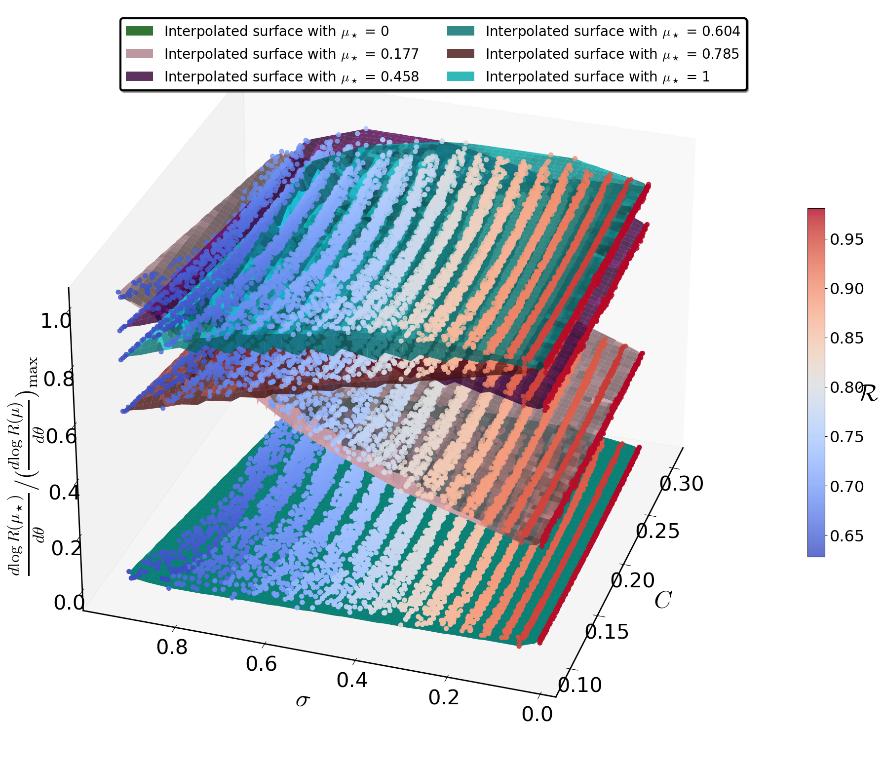
Universal description for fixed \(\mu\) values

x = 'C'; y = 'sigma'; w = 'Rpol/Req' ;z = 'dlogR_dtheta_scaled' ; z_model = '';

Surface_plot(df_new, x,y,w,z, xlabel=r'$C$',ylabel='$\sigma$',
                     wlabel = r'$\mathcal{R}$',
                     zlabel=r'$ \frac{d\log R(\mu_\star)}{d\theta}/(\frac{d\log R(\mu)}{d\theta})_{\mathrm{max}}$', 
                     view2=198, n_col=2, border_axes=1, X=None,Y=None,W = None,Z=None, l_w=1.5) #197

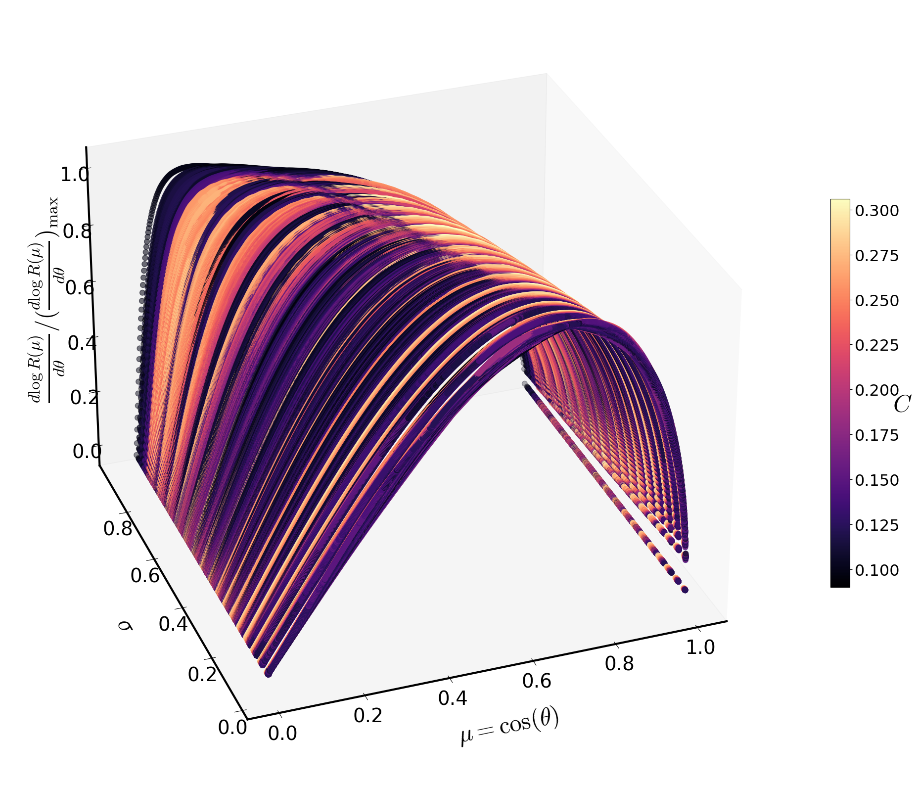
Universal description for each \(\mu\) value

fig = plt.figure(figsize=(20, 16))
labels_text_size = 40
ax = fig.add_subplot(111, projection='3d')
dot_size = 60
font_size = 35
label_pad = 35
label_size = 28

# 3D scatter plot
scatter = ax.scatter(mu_var, sigma_var, dlogR_min_max, c=C_var, cmap='magma', s=60) 

cbar = plt.colorbar(scatter,  shrink=0.5, )
cbar.set_label(r'$C$', fontsize=font_size,rotation = 0)
cbar.ax.tick_params(labelsize=23)

ax.view_init(30, 250)   
    

ax.set_xlabel(r'$\mu = \cos(\theta)$', fontsize=font_size,labelpad=label_pad) 
ax.set_ylabel(r'$\sigma$', fontsize=font_size,labelpad=label_pad) 

ax.zaxis.set_rotate_label(False)
ax.set_zlabel(r'$ \frac{d\log R(\mu)}{d\theta}/(\frac{d\log R(\mu)}{d\theta})_{\mathrm{max}}$', fontsize=font_size,labelpad=label_pad,rotation = 90) 
ax.zaxis.labelpad = 25
    
ax.xaxis.set_tick_params(labelsize=label_size)
ax.yaxis.set_tick_params(labelsize=label_size)
ax.zaxis.set_tick_params(labelsize=label_size)
    
for axis in [ax.xaxis, ax.yaxis, ax.zaxis]:
    axis.line.set_linewidth(3)
    
ax.grid(False)
plt.tight_layout()
plt.show()

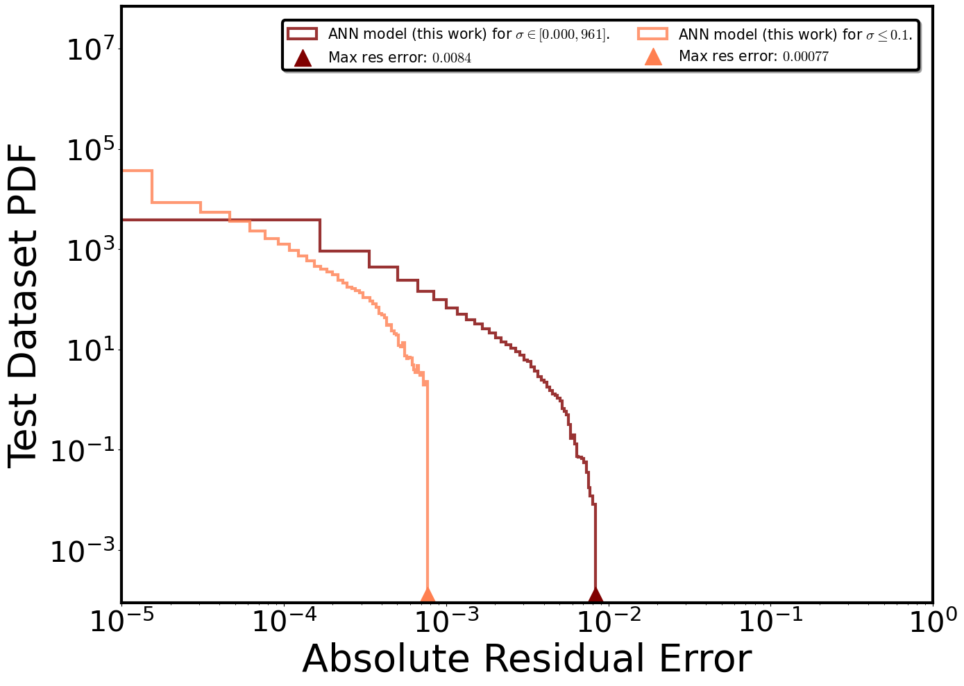
Percentage error histogram in the test set for the suggested ANN model’s optimal weights

ann_res = df['residual']

fig,ax = plt.subplots(figsize=(14, 10),)
labels_text_size = 40
plt.xticks(fontsize=30) #fontweight="bold"
plt.yticks(fontsize=30)

xlabel = r'Absolute Residual Error'
ylabel = r'Test Dataset PDF'

plt.xlabel(xlabel,size=labels_text_size)
plt.ylabel(ylabel,size=labels_text_size)

bins = 50
alpha = 0.8

# Histogram of errors aoociated with the proposed ANN Regression Model for at all sigma
y_reg_errors = (np.abs(df['residual'])).hist(
    density = True,
    lw =3,
    bins=bins,
    edgecolor ='maroon', 
    zorder = 1, 
    histtype='step',
    alpha = alpha, 
    label = 'ANN model (this work) for $\sigma \in [0.000,961]$.', color = 'maroon').autoscale(enable = True, axis = 'both', tight = True)

vertical_lines = [np.abs(df['residual']).max(), None]  # Adjust these values based on your requirements
plt.scatter(vertical_lines[0],1.25e-4, color='maroon', marker='^', s=300, zorder=2, label=f"Max res error: ${np.round(np.abs(ann_res).max(),4)}$")  # Star marker


# Histogram of errors aoociated with the proposed ANN Regression Model for sigma<=0.1
y_reg_errors_2 = (np.abs(df[df['sigma']<=0.1]['residual'])).hist(
    density = True,
    lw =3,
    bins=bins,
    edgecolor ='coral', 
    zorder = 1, 
    histtype='step',
    alpha = alpha, 
    label = 'ANN model (this work) for $\sigma \leq 0.1$.', color = 'coral').autoscale(enable = True, axis = 'both', tight = True)

vertical_lines = [np.abs(df[df['sigma']<=0.1]['residual']).max(), None]  # Adjust these values based on your requirements
plt.scatter(vertical_lines[0],1.25e-4, color='coral', marker='^', s=300, zorder=2, label=f"Max res error: ${np.round(np.abs(df[df['sigma']<=0.1]['residual']).max(),5)}$")  # Star marker


# Customize plot appearance
for axis in ['top', 'bottom', 'left', 'right']:
    ax.spines[axis].set_linewidth(3.0)


# Set logarithmic scale 
plt.xscale('log')
plt.yscale('log')


# Adjust x,y-axis limits (optional, based on log scale)
plt.xlim(0.1e-4,1)
plt.ylim(9e-5,70000000)



plt.grid(False)
leg = plt.legend(loc="upper right",ncol=2, borderaxespad=1, prop={'size': 14.7}, shadow=True, fontsize="large")    #,bbox_to_anchor=(1,1)
leg.get_frame().set_linewidth(3.0)
leg.get_frame().set_edgecolor('black')

plt.tight_layout()
plt.show()

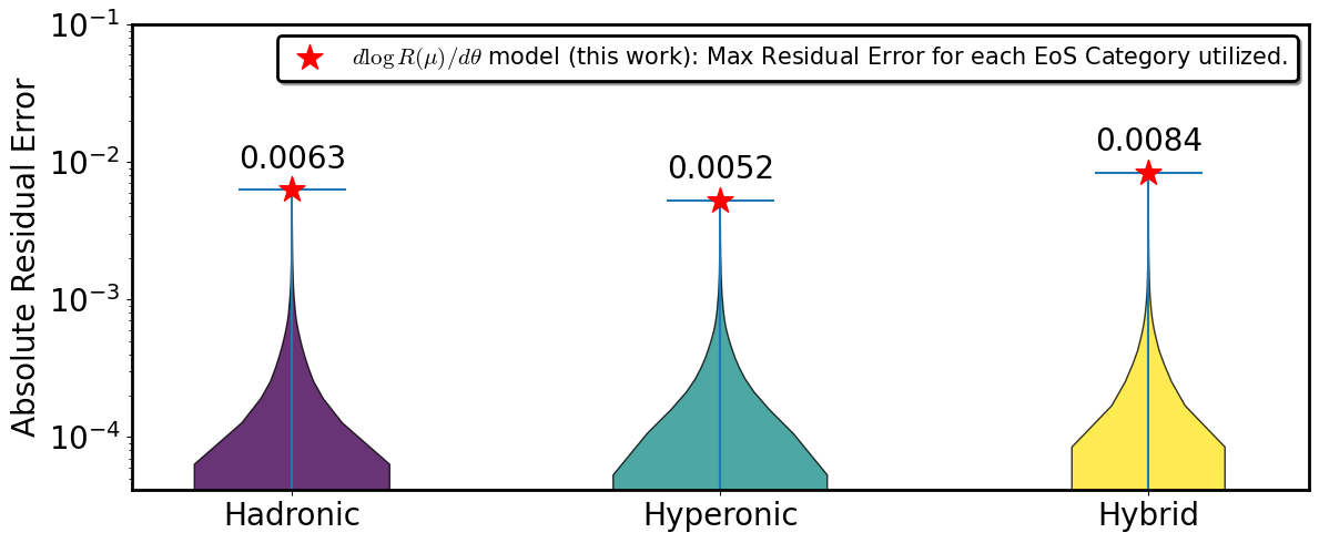
Distribution of absolute Residual Errors for each EoS category in the test set

eos_categories = ['Hadronic', 'Hyperonic', 'Hybrid']

EoS_categories_violin_plots(
    eos_categories = eos_categories, 
    df = df, 
    eval_metric = 'residual', 
    color_map = 'viridis', 
    label = r'$d \log R(\mu)/d \theta$ model (this work): Max Residual Error for each EoS Category utilized.', 
    scale = 'log',
    y_max = 1e-1,
    y_label = r"Absolute Residual Error")

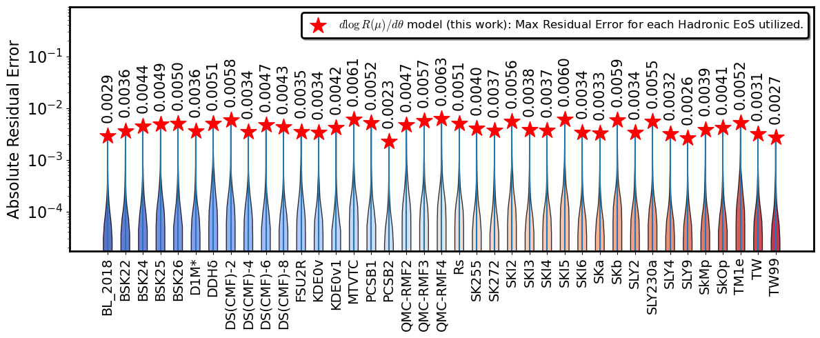
Distribution of absolute Relative Errors for Hadronic EoSs in the test set

eos_names = [ 'BL_2018', 'BSK22', 'BSK24', 'BSK25', 'BSK26', 'D1M*', 'DDHδ','DS(CMF)-2', 'DS(CMF)-4', 'DS(CMF)-6', 'DS(CMF)-8', 'FSU2R',
       'KDE0v', 'KDE0v1', 'MTVTC', 'PCSB1', 'PCSB2', 'QMC-RMF2','QMC-RMF3', 'QMC-RMF4', 'Rs', 'SK255', 'SK272', 'SKI2', 'SKI3',
       'SKI4', 'SKI5', 'SKI6', 'SKa', 'SKb', 'SLY2', 'SLY230a', 'SLY4', 'SLY9', 'SkMp', 'SkOp', 'TM1e', 'TW', 'TW99']


EoS_class_violin_plots(eos_names = eos_names, 
                 df = df, 
                 eval_metric = 'residual', 
                 eos_class = 'Hadronic EoSs', 
                 color_map = 'coolwarm', 
                 label = r'$d \log R(\mu)/d \theta$ model (this work): Max Residual Error for each Hadronic EoS utilized.', 
                 scale = 'log',      
                 y_max = 9e-1, 
                 y_label = r"Absolute Residual Error")

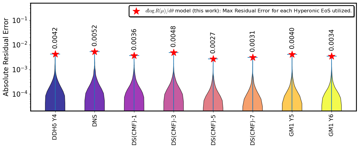
Distribution of absolute Relative Errors for Hyperonic EoSs in the test set

eos_names = [ 'DDHδ Υ4', 'DNS', 'DS(CMF)-1', 'DS(CMF)-3', 'DS(CMF)-5','DS(CMF)-7', 'GM1 Y5', 'GM1 Y6']

EoS_class_violin_plots(eos_names = eos_names, 
                 df = df, 
                 eval_metric = 'residual', 
                 eos_class = 'Hyperonic EoSs', 
                 color_map = 'plasma', 
                 label = r'$d \log R(\mu)/d \theta$ model (this work): Max Residual Error for each Hyperonic EoS utilized.', 
                 scale = 'log',      
                 y_max = 5e-1, 
                 y_label = r"Absolute Residual Error")

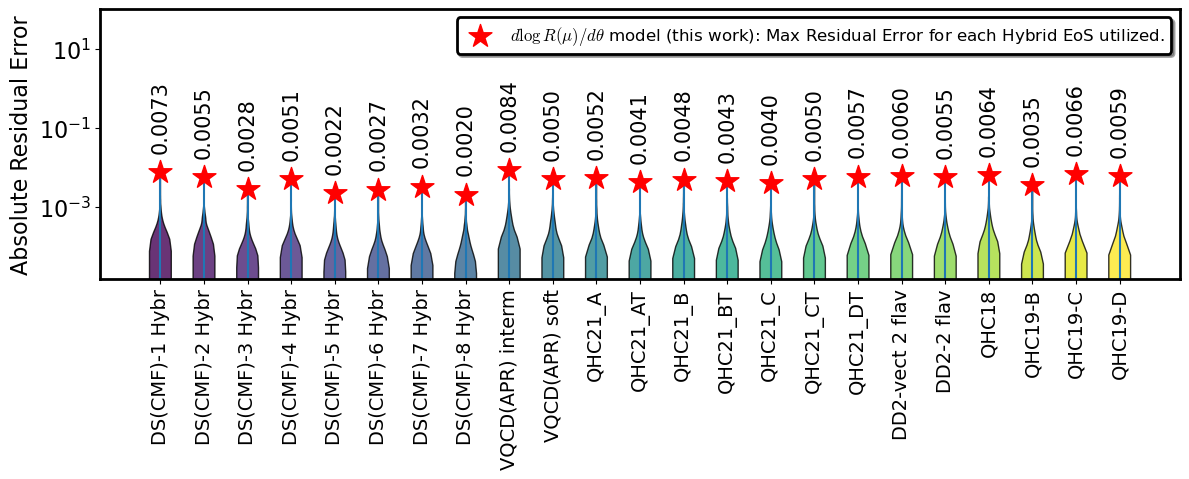
Distribution of absolute Relative Errors for Hybrid EoSs in the test set

eos_names = ['DS(CMF)-1 Hybrid', 'DS(CMF)-2 Hybrid', 'DS(CMF)-3 Hybrid','DS(CMF)-4 Hybrid', 'DS(CMF)-5 Hybrid', 'DS(CMF)-6 Hybrid',
       'DS(CMF)-7 Hybrid', 'DS(CMF)-8 Hybrid','JJ(VQCD(APR)), intermediate', 'JJ(VQCD(APR)), soft','KBH(QHC21_A)', 'KBH(QHC21_AT)', 'KBH(QHC21_B)', 'KBH(QHC21_BT)',
       'KBH(QHC21_C)', 'KBH(QHC21_CT)', 'KBH(QHC21_DT)','OOS(DD2)-vect interaction 2 flavors', 'OOS(DD2-FRG)-2 flavors',
       'QHC18', 'QHC19-B', 'QHC19-C', 'QHC19-D']


EoS_class_violin_plots(eos_names = eos_names, 
                 df = df, 
                 eval_metric = 'residual', 
                 eos_class = 'Hybrid EoSs', 
                 color_map = 'viridis', 
                 label = r'$d \log R(\mu)/d \theta$ model (this work): Max Residual Error for each Hybrid EoS utilized.', 
                 scale = 'log',      
                 y_max = 100, 
                 y_label = r"Absolute Residual Error")

ANN Regression Model for the star’s Logarithmic derivative at surface: Evaluation on singular EOS

# Choose the case/EoS of your preference
# In this demo we provide indicatively for demonstration 3 EoS: 1 per star's category investigated

# Hadronic case
#file_name = './Surface models for Hadronic EOS/SLY4/'

# Hyperonic case
#file_name = './Surface models for Hyperonic EOS/DNS/'

# Hybrid case
file_name = './Surface models for Hybrid EOS/KBH(QHC21_AT)/'

spin = 'sigma' 
test_percentage = 0.2

rotational_path = os.path.join(file_name, 'rotational_models.zip')
static_path = os.path.join(file_name, 'static_models.zip')

df_rot_train, df_rot_test = read_zip(rotational_path, spin=spin, test_percentage=test_percentage)
df_stat_train, df_stat_test = read_zip(static_path, spin=spin, test_percentage=test_percentage)

df_train = pd.concat([df_rot_train, df_stat_train], ignore_index=True)
df_test = pd.concat([df_rot_test, df_stat_test], ignore_index=True)

# Free the memory space
del df_rot_train, df_rot_test, df_stat_train, df_stat_test

Load the Trained Regression Model optimal weights to estimate the Logarithmic derivative at the star’s surface

batch_size = 4096
model_path = './Model/Derivative/Derivative-model.pth'

dataloader_tr, input_dimension, np_features_tr, np_targets_tr = load_stars(df_train, batch_size=batch_size)
dataloader_ts, _, np_features_ts, np_targets_ts = load_stars(df_test, batch_size=batch_size)

regressor = Regressor(input_dimension=input_dimension, feature_scaler=feature_scaler).to(device)
regressor.set_device(device)
regressor.load_state_dict(torch.load(model_path, map_location=torch.device(device)))
regressor.eval()

Regressor(
  (MLP): Sequential(
    (0): Linear(in_features=4, out_features=200, bias=True)
    (1): LeakyReLU(negative_slope=0.1, inplace=True)
    (2): Linear(in_features=200, out_features=100, bias=True)
    (3): LeakyReLU(negative_slope=0.1, inplace=True)
    (4): Linear(in_features=100, out_features=50, bias=True)
    (5): LeakyReLU(negative_slope=0.1, inplace=True)
    (6): Linear(in_features=50, out_features=25, bias=True)
    (7): LeakyReLU(negative_slope=0.1, inplace=True)
    (8): Linear(in_features=25, out_features=10, bias=True)
    (9): LeakyReLU(negative_slope=0.1, inplace=True)
    (10): Linear(in_features=10, out_features=1, bias=True)
    (11): Sigmoid()
  )
)

Plot functions associated with residual and percentage errors

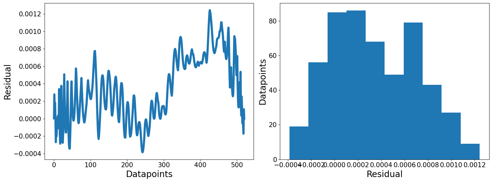
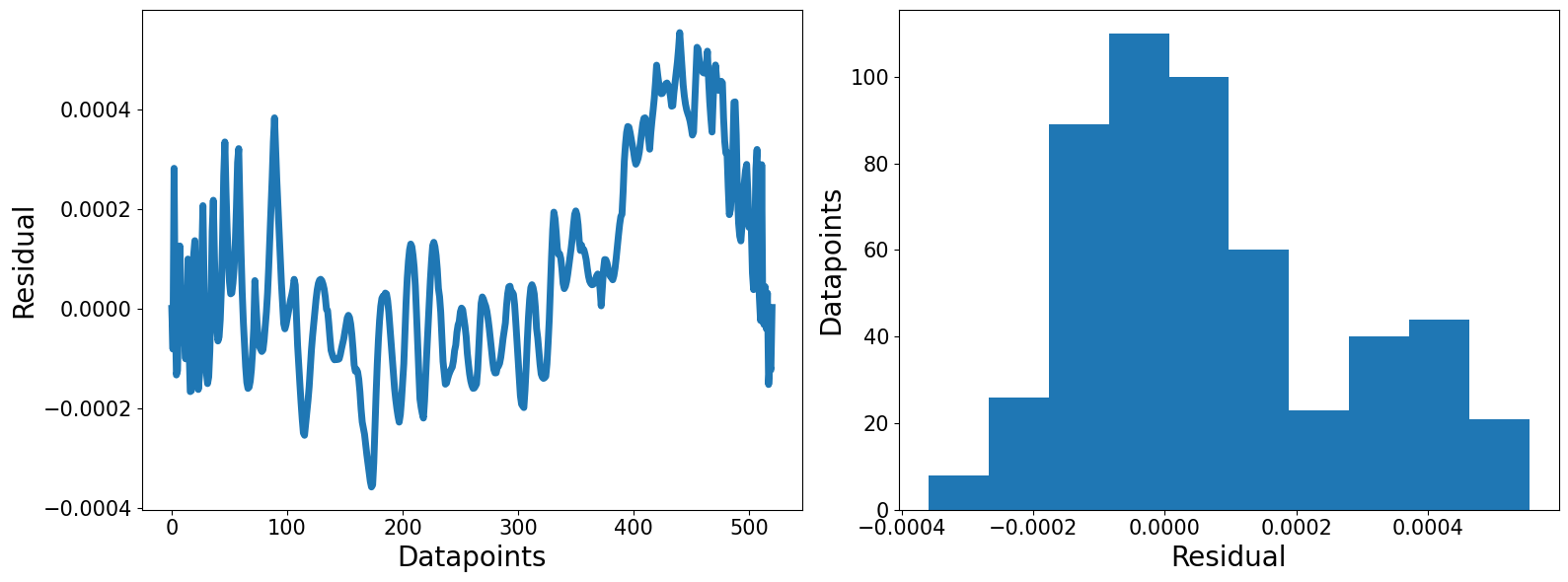
def plot_residuals(residual_error):
    witdh, height = 16, 6
    fontsize = 20
    labelsize = 15
    lw = 5
    
    fig, ax = plt.subplots(1, 2, figsize=(witdh, height))
    # Residual error subplot 
    ax[0].plot(residual_error, lw=lw)
    ax[0].set_xlabel(r'Datapoints', fontsize=fontsize)
    ax[0].set_ylabel(r'Residual', fontsize=fontsize)
    ax[0].tick_params(axis='both', which='both', labelsize=labelsize)
   
    ax[1].hist(residual_error, lw=lw)
    ax[1].set_ylabel(r'Datapoints', fontsize=fontsize)
    ax[1].set_xlabel(r'Residual', fontsize=fontsize)
    ax[1].tick_params(axis='both', which='both', labelsize=labelsize)

    plt.tight_layout()
    plt.show()

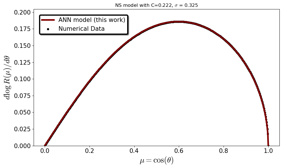
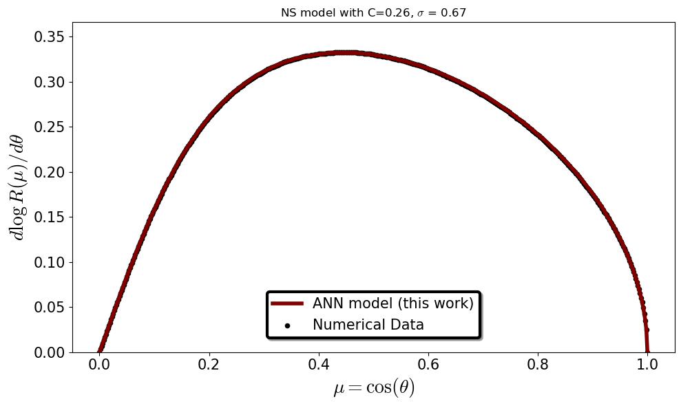
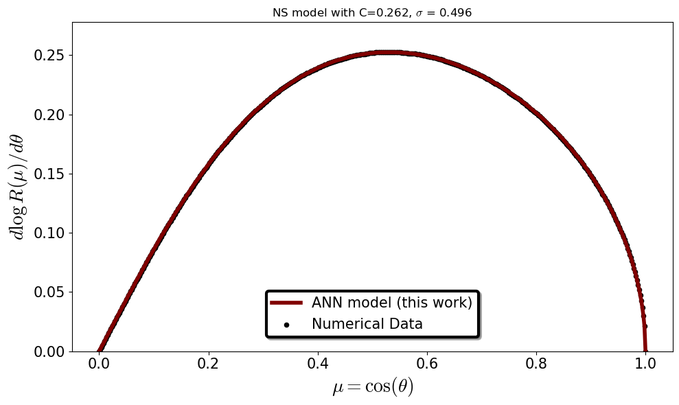
def plot_derivative(mu, model_estimation, real_targets, C, sigma):
    witdh, height = 10, 6
    fontsize = 20
    labelsize = 15
    lw = 4

    fig, ax = plt.subplots(figsize=(witdh, height))
    ax.plot(mu, model_estimation, lw=lw, c='maroon', label='ANN model (this work)')
    ax.scatter(mu, real_targets, c='black', s=20, marker='o', label='Numerical Data')
    plt.ylim((1-0.1)*real_targets.min(), (1+0.1)*real_targets.max())
    plt.xlabel(r'$\mu = \cos(\theta)$', fontsize=fontsize)
    plt.ylabel(r'$d\log R(\mu)/d\theta$', fontsize=fontsize)
    plt.title(f'NS model with C={round(C,3)}, $\sigma$ = {round(sigma,3)}')
    plt.legend(loc='best', prop={'size':fontsize}, shadow=True, fontsize='large')
    ax.tick_params(axis='both', which='both', labelsize=labelsize)

    leg = plt.legend(loc="best", ncol=1, borderaxespad=1, prop={'size': 15.},  shadow=True, fontsize="large")
    leg.get_frame().set_linewidth(3.0)
    leg.get_frame().set_edgecolor('black')
    plt.tight_layout()
    plt.show()

Universal relations suggested in this work for the parameters \(e\), \(R_p/R_e\) and \((d\log R/d \theta)_{\mathrm{max}}\)

#def eccentricity(C, sigma):
#    return (
#        -99.173162625833 * C**5 +68.055729822908 * C**4 * sigma + 137.191420602024 * C**4 +12.9349885313244 * C**3 * sigma**2 -
#        57.474308297241 * C**3 * sigma -67.7948794729071 * C**3 -9.03315944594535 * C**2 * sigma**3 + 8.08346062523145 * C**2 * sigma**2 +
#        9.19713339469957 * C**2 * sigma + 14.9006458417145 * C**2 + 4.84885244516378 * C * sigma**4 -
#        6.44626099699536 * C * sigma**3 +2.75499036217858 * C * sigma**2 -
#        1.3329369261108 * C * sigma - 1.52533604289959 * C + 4.71450473450295 * sigma**5 -
#        13.8547513636472 * sigma**4 + 15.4712200610891 * sigma**3 - 8.71280504897915 * sigma**2 +
#        3.0422989983075 * sigma + 0.182560763719325
#    )

#def R_pole(R_e, C, sigma):
#    return (
#        R_e*(-45.3015234274801 * C**4 - 7.52466249012259 * C**3 * sigma
#        + 36.1318805958812 * C**3 - 2.50668582910242 * C**2 * sigma**2
#        + 8.66838156199219 * C**2 * sigma - 10.4561101976216 * C**2
#        + 0.527775373801867 * C * sigma**3 - 0.226904263928412 * C * sigma**2
#        - 1.45892092679705 * C * sigma + 1.29663161750561 * C + 0.196118434593753 * sigma**4
#        - 0.440968195037673 * sigma**3 + 0.544639042230603 * sigma**2 - 0.617710700567153 * sigma
#        + 0.942328028476575)
#    )    

#def dLogR_dtheta_Max(C, sigma, R):
#    return (
#        -0.403276601295374 * C**3 +0.661519097793562 * C**2 * sigma +
#        2.57434191155828 * C**2 * R -2.23108454811518 * C**2 -
#        8.67625739742325 * C * sigma**2 - 39.6796750693722 * C * sigma * R +
#        38.4663786235779 * C * sigma - 45.0567823427512 * C * R**2 +
#        87.0956609308423 * C * R - 42.1349805655397 * C +
#        4.07991541887412 * sigma**3 + 30.4880078788823 * sigma**2 * R -
#        27.2418077134724 * sigma**2 + 72.1353182129003 * sigma * R**2 -
#        130.455828718591 * sigma * R + 58.5590616356724 * sigma +
#        53.9663039265715 * R**3 - 146.858522848505 * R**2 +
#        131.341936932855 * R - 38.4414384733067
#    )

Select NS for estimating the LOgarithmic derivative with the associated residuals

# Select Set (Train/Test)
is_train = True # True or False

# Select your favourite Star
star_index = 1

# Do not change
low = star_index * N_MU
high = (star_index + 1) * N_MU

select_set = lambda is_train, df_train, df_test: df_train if is_train else df_test
select_features = lambda is_train, np_features_tr, np_features_ts: np_features_tr if is_train else np_features_ts
select_targets = lambda is_train, np_targets_tr, np_targets_ts: np_targets_tr if is_train else np_targets_ts
    
# Select Set (Train/Test)
df_set = select_set(is_train, df_train, df_test)
features = select_features(is_train, np_features_tr, np_features_ts)
targets = select_targets(is_train, np_targets_tr, np_targets_ts)

# Model's log-der estimation using the suggested ANN model
estimation = regressor.predict(features[low:high]).ravel().astype(np.float64) 
max_ = df_set['dlogR_dtheta'].iloc[low:high].max()

##########################################################
# max_ taken from the universal relation suggested
#C = df_set['C'].iloc[low]
#sigma =  df_set['sigma'].iloc[low]
#R_e = df_set['Req_num'].iloc[low]
#r_star = R_pole(R_e, C, sigma)/R_e
#max_ = dLogR_dtheta_Max(C, sigma, r_star)
###########################################################

# Static case
model_estimation = estimation * max_ 
real_targets = targets[low:high] * max_

real_targets = real_targets.ravel().astype(np.float64) 
    
mu = df_set['cos(theta)'].iloc[low:high]

Residual error computation

residual_error = model_estimation - real_targets

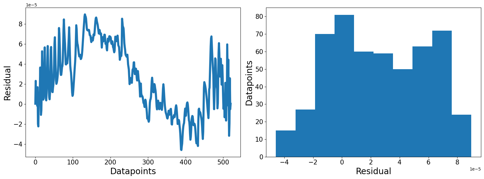
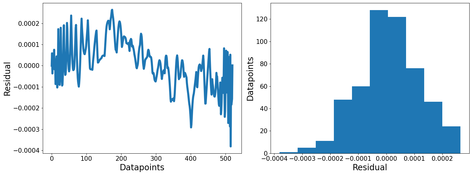
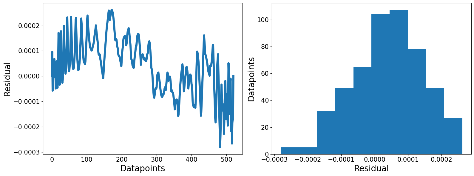
Error distributions for the logarithmic derivative at surface of singular NS configuration

plot_residuals(residual_error)

Logarithmic derivative at surface for an indicative NS configuration

plot_derivative(mu, model_estimation, real_targets, df_set['C'].iloc[low], df_set['sigma'].iloc[low])

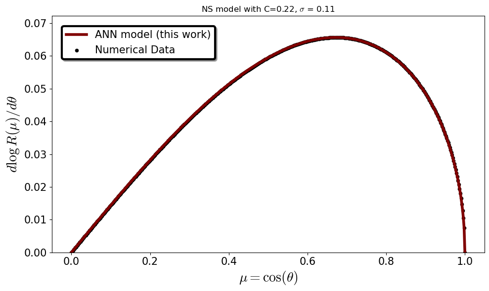
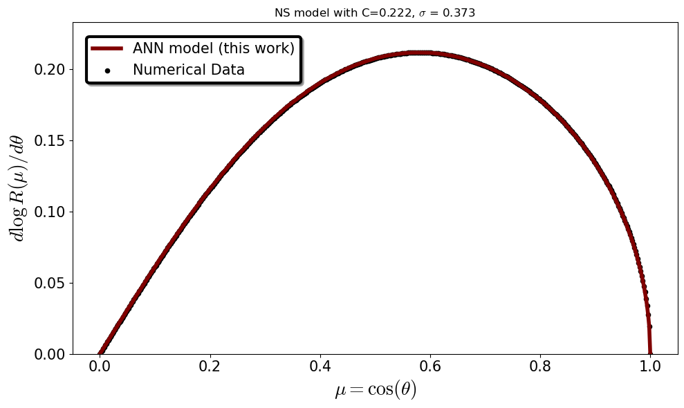
Visualization of the all the log-derivative curves in the selected set (Train/Test) dataset for the specific EOS loaded

# Select Training or test set
is_train = False # True or False

select_set = lambda is_train, df_train, df_test: df_train if is_train else df_test
select_features = lambda is_train, np_features_tr, np_features_ts: np_features_tr if is_train else np_features_ts
select_targets = lambda is_train, np_targets_tr, np_targets_ts: np_targets_tr if is_train else np_targets_ts
    
# Select Set (Train/Test)
df_set = select_set(is_train, df_train, df_test)
features = select_features(is_train, np_features_tr, np_features_ts)
targets = select_targets(is_train, np_targets_tr, np_targets_ts)
    
for star_index in range(0, 100):
    # Do not change
    low = star_index * N_MU
    high = (star_index + 1) * N_MU
    
    ############# C and sigma for each star ######################################
    C = df_set['C'].iloc[low]
    sigma = df_set['sigma'].iloc[low]
    R_e = df_set['Req_num'].iloc[low]
    ##############################################################################
    
   # Select and estimate star surface
    estimation = regressor.predict(features[low:high]).ravel().astype(np.float64) 
    max_ = df_set['dlogR_dtheta'].iloc[low:high].max()
    
    ##########################################################
    # max_ taken from universal relation extracted
    #r_star = R_pole(R_e, C, sigma)/R_e
    #max_ = dLogR_dtheta_Max(C, sigma, r_star)
    ###########################################################
    
    
    model_estimation = estimation * max_ 
    real_targets = targets[low:high] * max_

    real_targets = real_targets.ravel().astype(np.float64) 
    mu = df_set['cos(theta)'].iloc[low:high]
    
    residual_error = model_estimation - real_targets
    
    plot_residuals(residual_error)
    plot_derivative(mu, model_estimation, real_targets, C, sigma)

---------------------------------------------------------------------------
AttributeError                            Traceback (most recent call last)
File ~/anaconda3/lib/python3.11/site-packages/PIL/ImageFile.py:536, in _save(im, fp, tile, bufsize)
    535 try:
--> 536     fh = fp.fileno()
    537     fp.flush()

AttributeError: '_idat' object has no attribute 'fileno'

During handling of the above exception, another exception occurred:

KeyboardInterrupt                         Traceback (most recent call last)
Cell In[35], line 43
     39 mu = df_set['cos(theta)'].iloc[low:high]
     41 residual_error = model_estimation - real_targets
---> 43 plot_residuals(residual_error)
     44 plot_derivative(mu, model_estimation, real_targets, C, sigma)

Cell In[28], line 20, in plot_residuals(residual_error)
     17 ax[1].tick_params(axis='both', which='both', labelsize=labelsize)
     19 plt.tight_layout()
---> 20 plt.show()

File ~/anaconda3/lib/python3.11/site-packages/matplotlib/pyplot.py:527, in show(*args, **kwargs)
    483 """
    484 Display all open figures.
    485 
   (...)
    524 explicitly there.
    525 """
    526 _warn_if_gui_out_of_main_thread()
--> 527 return _get_backend_mod().show(*args, **kwargs)

File ~/anaconda3/lib/python3.11/site-packages/matplotlib_inline/backend_inline.py:90, in show(close, block)
     88 try:
     89     for figure_manager in Gcf.get_all_fig_managers():
---> 90         display(
     91             figure_manager.canvas.figure,
     92             metadata=_fetch_figure_metadata(figure_manager.canvas.figure)
     93         )
     94 finally:
     95     show._to_draw = []

File ~/anaconda3/lib/python3.11/site-packages/IPython/core/display_functions.py:298, in display(include, exclude, metadata, transient, display_id, raw, clear, *objs, **kwargs)
    296     publish_display_data(data=obj, metadata=metadata, **kwargs)
    297 else:
--> 298     format_dict, md_dict = format(obj, include=include, exclude=exclude)
    299     if not format_dict:
    300         # nothing to display (e.g. _ipython_display_ took over)
    301         continue

File ~/anaconda3/lib/python3.11/site-packages/IPython/core/formatters.py:179, in DisplayFormatter.format(self, obj, include, exclude)
    177 md = None
    178 try:
--> 179     data = formatter(obj)
    180 except:
    181     # FIXME: log the exception
    182     raise

File ~/anaconda3/lib/python3.11/site-packages/decorator.py:232, in decorate.<locals>.fun(*args, **kw)
    230 if not kwsyntax:
    231     args, kw = fix(args, kw, sig)
--> 232 return caller(func, *(extras + args), **kw)

File ~/anaconda3/lib/python3.11/site-packages/IPython/core/formatters.py:223, in catch_format_error(method, self, *args, **kwargs)
    221 """show traceback on failed format call"""
    222 try:
--> 223     r = method(self, *args, **kwargs)
    224 except NotImplementedError:
    225     # don't warn on NotImplementedErrors
    226     return self._check_return(None, args[0])

File ~/anaconda3/lib/python3.11/site-packages/IPython/core/formatters.py:340, in BaseFormatter.__call__(self, obj)
    338     pass
    339 else:
--> 340     return printer(obj)
    341 # Finally look for special method names
    342 method = get_real_method(obj, self.print_method)

File ~/anaconda3/lib/python3.11/site-packages/IPython/core/pylabtools.py:152, in print_figure(fig, fmt, bbox_inches, base64, **kwargs)
    149     from matplotlib.backend_bases import FigureCanvasBase
    150     FigureCanvasBase(fig)
--> 152 fig.canvas.print_figure(bytes_io, **kw)
    153 data = bytes_io.getvalue()
    154 if fmt == 'svg':

File ~/anaconda3/lib/python3.11/site-packages/matplotlib/backend_bases.py:2187, in FigureCanvasBase.print_figure(self, filename, dpi, facecolor, edgecolor, orientation, format, bbox_inches, pad_inches, bbox_extra_artists, backend, **kwargs)
   2183 try:
   2184     # _get_renderer may change the figure dpi (as vector formats
   2185     # force the figure dpi to 72), so we need to set it again here.
   2186     with cbook._setattr_cm(self.figure, dpi=dpi):
-> 2187         result = print_method(
   2188             filename,
   2189             facecolor=facecolor,
   2190             edgecolor=edgecolor,
   2191             orientation=orientation,
   2192             bbox_inches_restore=_bbox_inches_restore,
   2193             **kwargs)
   2194 finally:
   2195     if bbox_inches and restore_bbox:

File ~/anaconda3/lib/python3.11/site-packages/matplotlib/backend_bases.py:2043, in FigureCanvasBase._switch_canvas_and_return_print_method.<locals>.<lambda>(*args, **kwargs)
   2039     optional_kws = {  # Passed by print_figure for other renderers.
   2040         "dpi", "facecolor", "edgecolor", "orientation",
   2041         "bbox_inches_restore"}
   2042     skip = optional_kws - {*inspect.signature(meth).parameters}
-> 2043     print_method = functools.wraps(meth)(lambda *args, **kwargs: meth(
   2044         *args, **{k: v for k, v in kwargs.items() if k not in skip}))
   2045 else:  # Let third-parties do as they see fit.
   2046     print_method = meth

File ~/anaconda3/lib/python3.11/site-packages/matplotlib/backends/backend_agg.py:497, in FigureCanvasAgg.print_png(self, filename_or_obj, metadata, pil_kwargs)
    450 def print_png(self, filename_or_obj, *, metadata=None, pil_kwargs=None):
    451     """
    452     Write the figure to a PNG file.
    453 
   (...)
    495         *metadata*, including the default 'Software' key.
    496     """
--> 497     self._print_pil(filename_or_obj, "png", pil_kwargs, metadata)

File ~/anaconda3/lib/python3.11/site-packages/matplotlib/backends/backend_agg.py:446, in FigureCanvasAgg._print_pil(self, filename_or_obj, fmt, pil_kwargs, metadata)
    441 """
    442 Draw the canvas, then save it using `.image.imsave` (to which
    443 *pil_kwargs* and *metadata* are forwarded).
    444 """
    445 FigureCanvasAgg.draw(self)
--> 446 mpl.image.imsave(
    447     filename_or_obj, self.buffer_rgba(), format=fmt, origin="upper",
    448     dpi=self.figure.dpi, metadata=metadata, pil_kwargs=pil_kwargs)

File ~/anaconda3/lib/python3.11/site-packages/matplotlib/image.py:1656, in imsave(fname, arr, vmin, vmax, cmap, format, origin, dpi, metadata, pil_kwargs)
   1654 pil_kwargs.setdefault("format", format)
   1655 pil_kwargs.setdefault("dpi", (dpi, dpi))
-> 1656 image.save(fname, **pil_kwargs)

File ~/anaconda3/lib/python3.11/site-packages/PIL/Image.py:2439, in Image.save(self, fp, format, **params)
   2436         fp = builtins.open(filename, "w+b")
   2438 try:
-> 2439     save_handler(self, fp, filename)
   2440 except Exception:
   2441     if open_fp:

File ~/anaconda3/lib/python3.11/site-packages/PIL/PngImagePlugin.py:1402, in _save(im, fp, filename, chunk, save_all)
   1398     im = _write_multiple_frames(
   1399         im, fp, chunk, rawmode, default_image, append_images
   1400     )
   1401 if im:
-> 1402     ImageFile._save(im, _idat(fp, chunk), [("zip", (0, 0) + im.size, 0, rawmode)])
   1404 if info:
   1405     for info_chunk in info.chunks:

File ~/anaconda3/lib/python3.11/site-packages/PIL/ImageFile.py:540, in _save(im, fp, tile, bufsize)
    538     _encode_tile(im, fp, tile, bufsize, fh)
    539 except (AttributeError, io.UnsupportedOperation) as exc:
--> 540     _encode_tile(im, fp, tile, bufsize, None, exc)
    541 if hasattr(fp, "flush"):
    542     fp.flush()

File ~/anaconda3/lib/python3.11/site-packages/PIL/ImageFile.py:559, in _encode_tile(im, fp, tile, bufsize, fh, exc)
    556 if exc:
    557     # compress to Python file-compatible object
    558     while True:
--> 559         errcode, data = encoder.encode(bufsize)[1:]
    560         fp.write(data)
    561         if errcode:

KeyboardInterrupt: