

RNS in a notebook — a hands-on tour of rapidly rotating relativistic stars#
Code: RNS v1.1e (N. Stergioulas) Method: KEH (Komatsu–Eriguchi–Hachisu 1989) with CST (Cook–Shapiro–Teukolsky 1992, 1994a,b) modifications Papers reproduced here: Stergioulas & Friedman 1995 (ApJ 444, 306); Nozawa, Stergioulas, Gourgoulhon & Eriguchi 1998 (A&AS 132, 431)
RNS is a C executable that solves Einstein’s equations coupled to hydrostationary equilibrium for uniformly rotating, axisymmetric, perfect-fluid stars. This notebook drives it from Pythonvia a thin wrapper (rns_helpers.py), parses the output, and walks through the main classes of applications: single models, sequences, the two-dimensional surface of equilibria in \((M, J, \varepsilon_c)\), and several astrophysical use cases.
Most cells finish in seconds at the default 65×129 grid; the cells flagged (slow) can take up to a few minutes.
1. Setup#
The wrapper expects an rns_build/ directory containing the compiled binaries rns, rns_high, rns_vh, ‘rns_xh’, hng and the bundled eos/ directory. On a fresh machine:
git clone https://gitlab.com/niksterg/acme-rns.git
cd rns_build
make
The cell below verifies the build and applies a uniform matplotlib style.
import os, sys, time
from pathlib import Path
import numpy as np
import pandas as pd
import matplotlib.pyplot as plt

# Tell rns_helpers where to find the binaries
os.environ.setdefault("RNS_BUILD_DIR", str(Path("rns_build").resolve()))

import rns_helpers as rh
rh.apply_paper_style()

print("RNS build dir :", rh.BUILD_DIR)
for g in ("std", "high", "vh", "xh"):
    try:
        print(f"  binary [{g:>4}] :", rh._binary(g))
    except FileNotFoundError as e:
        print(f"  binary [{g:>4}] : MISSING -- {e}")
print("  binary [ hng] :", rh._binary("hng"))
RNS build dir : /Users/niksterg/Repositories/GITLAB/niksterg/acme-rns/rns_build
  binary [ std] : /Users/niksterg/Repositories/GITLAB/niksterg/acme-rns/rns_build/rns
  binary [high] : /Users/niksterg/Repositories/GITLAB/niksterg/acme-rns/rns_build/rns_high
  binary [  vh] : /Users/niksterg/Repositories/GITLAB/niksterg/acme-rns/rns_build/rns_vh
  binary [  xh] : /Users/niksterg/Repositories/GITLAB/niksterg/acme-rns/rns_build/rns_xh
  binary [ hng] : /Users/niksterg/Repositories/GITLAB/niksterg/acme-rns/rns_build/hng
1.1 A collection of legacy EOS table#
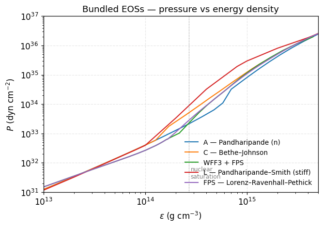
The bundled EOSs span the range from soft (G, Canuto–Chitre — too soft to support the observed ≈2 M\(_\odot\) pulsars but useful as a numerical stress test) to extremely stiff (L, Pandharipande–Smith). The plot below shows \(P\) vs \(\varepsilon\) on log–log axes for the six EOSs we use throughout this notebook. The slope is the polytropic exponent \(\Gamma = d\ln P / d\ln \varepsilon\) — note how the high-density slope differs between EOSs; this is exactly what drives the maximum-mass and Kepler-limit differences we’ll see later.
EOS_LIST = ["eosA", "eosC", "eosWS", "eosL", "eosFPS"]
EOS_LABELS = {
    "eosA":   "A — Pandharipande (n)",
    "eosC":   "C — Bethe–Johnson",
    "eosWS":  "WFF3 + FPS",
    "eosL":   "L — Pandharipande–Smith (stiff)",
    "eosFPS": "FPS — Lorenz–Ravenhall–Pethick",
}

fig, ax = plt.subplots(figsize=(6.2, 4.4))
for eos in EOS_LIST:
    tab = rh.load_eos(eos)
    ax.loglog(tab["epsilon"], tab["P"], label=EOS_LABELS[eos])
ax.set_xlabel(r"$\varepsilon$ (g cm$^{-3}$)")
ax.set_ylabel(r"$P$ (dyn cm$^{-2}$)")
ax.set_xlim(1e13, 5e15); ax.set_ylim(1e31, 1e37)
ax.axvline(2.7e14, color='gray', ls=':', lw=0.8)
ax.text(2.8e14, 3e31, "nuclear\nsaturation", fontsize=8, color='gray')
ax.legend(loc='lower right', frameon=False)
ax.set_title("Bundled EOSs — pressure vs energy density")
plt.tight_layout(); plt.show()
2. A first model — anatomy of an RNS run#
We reproduce Example 1 from examples.test: EOS C, central energy density \(\varepsilon_c = 2 \times 10^{15}\) g cm\(^{-3}\), axes ratio \(r_p/r_e = 0.59\). Specifying the axes ratio with -r is the fastest path — RNS solves one boundary-value problem and stops. Every other task internally varies the axes ratio to hit a requested mass, rate, etc.
res = rh.run_rns(task="model", eos="eosC", e=2e15, r=0.59)
print(f"  {'quantity':14s}  {'value':12s}  unit")
for quantity, value, unit in rh.parse_p1_rows(res.raw):
    print(f"  {quantity:14s}  {value:12.6g}  {unit}")
  quantity        value         unit
  e_c                        2  10^15 g/cm^3
  M                    2.13324  M_sun
  M_0                  2.43446  M_sun
  R_e                  13.9518  km
  Omega               0.961702  10^4 s^-1
  Omega_p              1.00322  10^4 s^-1
  T/W                 0.109774
  cJ/GM_sun^2          2.89653
  I                    2.64698  10^45 g cm^2
  h+                  0.129382  km
  h-                   11.9949  km
  Z_p                 0.591305
  Z_f                -0.296001
  Z_b                  1.66307
  omega_c/Omega       0.722768
  r_e                  10.4129  km
  r_p/r_e                 0.59
  GRV2                0.020401
  GRV3             0.000935058
Note that we follow the convention of reporting the energy densit \(\epsilon\) as \(\epsilon/c^2\), so in units of \({\rm g}/{\rm cm}^3\) !
Reading the output. All 17 quantities printed by RNS have direct physical meaning. Tying them to the GR notes:
\(M, M_0\) — gravitational (ADM) and rest masses, computed as Komar-type integrals over the source. The difference \(M_0 + U + T - M\) is the gravitational binding energy.
\(R_e\) — the circumferential equatorial radius \(R_e = e^{\psi}|_{\theta=\pi/2}\). This is the radius that enters the redshift, not the coordinate \(r_e\).
\(\Omega\) — the constant angular velocity as seen from infinity. \(\Omega_p\) is the Keplerian angular velocity of a test particle in circular orbit at the equator; the star is at the mass-shed limit when \(\Omega \to \Omega_p\).
\(T/W\) — rotational/binding-energy ratio; a fast diagnostic for whether the star is near the secular or dynamical bar instability.
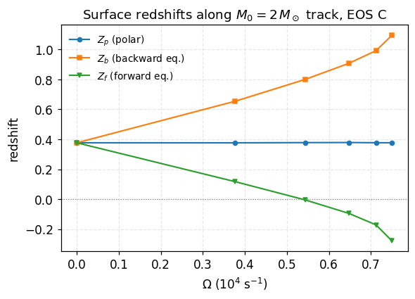
\(Z_p, Z_f, Z_b\) — polar and equatorial forward/backward redshifts. The forward redshift can be negative — that is a blueshift, because the equatorial fluid on the approaching side is moving towards us faster than the gravitational redshift can slow it.
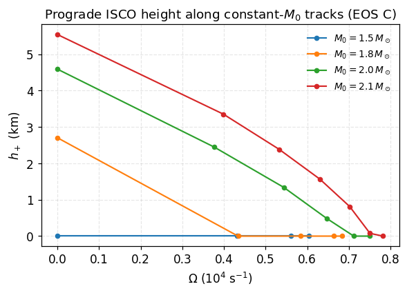
\(h_+, h_-\) — heights of the prograde / retrograde innermost stable circular orbits above the surface. \(h_+ = 0\) (as here for many stars with low mass and/or near mass-shed) means all prograde orbits down to the surface are stable.
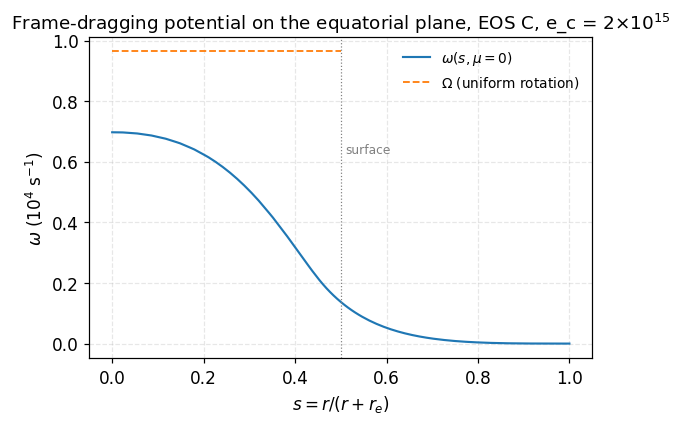
\(\omega_c/\Omega\) — central frame-dragging rate, normalized by the angular velocity of the star.
3. RNS tasks#
RNS specifies a model uniquely by two parameters: always the central energy density \(\varepsilon_c\), and one of {axes ratio, \(M\), \(M_0\), \(\Omega\), \(J\)}. There are seven tasks:
task |
flag combination |
what it fixes |
|---|---|---|
|
|
\(\varepsilon_c\), \(\Omega=0\) (TOV) |
|
|
\(\varepsilon_c\) and axes ratio (fastest) |
|
|
\(\varepsilon_c\) and gravitational mass |
|
|
\(\varepsilon_c\) and rest (baryon) mass |
|
|
\(\varepsilon_c\) and angular velocity |
|
|
\(\varepsilon_c\) and angular momentum |
|
|
\(\varepsilon_c\), \(\Omega = \Omega_K\) |
Every task other than model and static is solved iteratively by varying \(r_p/r_e\) until the requested second parameter falls within fix_error (default \(10^{-4}\)). The next four cells produce the same star from four different specifications.
# Static (TOV) reference
ref_static = rh.run_rns(task="static", eos="eosC", e=1e15)
print(f"TOV at e_c = 1e15 g/cm^3:  M = {ref_static['M']:.4f} M_sun,  R = {ref_static['R_e']:.3f} km")
TOV at e_c = 1e15 g/cm^3: M = 1.3250 M_sun, R = 12.007 km
# Now spin it up four ways at the same e_c. Specify each task's required parameter
# from one prior model so the answers must agree.

# (a) by axes ratio
a = rh.run_rns(task="model",   eos="eosC", e=1e15, r=0.75)
# (b) by gravitational mass (use a's M)
b = rh.run_rns(task="gmass",   eos="eosC", e=1e15, M=a["M"])
# (c) by angular velocity   (use a's Omega)
c = rh.run_rns(task="omega",   eos="eosC", e=1e15, Omega=a["Omega"])
# (d) by angular momentum   (use a's cJ/GM^2)
d = rh.run_rns(task="jmoment", eos="eosC", e=1e15, J=a["cJ_GMsun2"])

cmp = pd.DataFrame(
    {"by r_p/r_e": a.data, "by gmass": b.data, "by omega": c.data, "by J": d.data}
).T[["M","M_0","R_e","Omega","cJ_GMsun2","T_W","r_ratio"]]
cmp.round(5)
| M | M_0 | R_e | Omega | cJ_GMsun2 | T_W | r_ratio | |
|---|---|---|---|---|---|---|---|
| by r_p/r_e | 1.51163 | 1.65345 | 13.8945 | 0.57990 | 1.20012 | 0.06797 | 0.75 |
| by gmass | 1.51169 | 1.65352 | 13.8947 | 0.57989 | 1.20017 | 0.06797 | 0.75 |
| by omega | 1.51169 | 1.65352 | 13.8947 | 0.57989 | 1.20017 | 0.06797 | 0.75 |
| by J | 1.51169 | 1.65352 | 13.8947 | 0.57989 | 1.20017 | 0.06797 | 0.75 |
The four reconstructions agree to ~\(10^{-4}\) — the default fix_error tolerance. You can tighten it with the fix_error= argument if you need more precision (at the cost of more iterations), but this is meaningful if the grid resolution is also increased.
3.1 The mass-shed (Kepler) limit#
-t kepler increases the rotation rate until the equator co-rotates with a test particle in circular orbit, \(\Omega = \Omega_p\). At that point no further uniform rotation is possible: adding angular momentum sheds mass off the equator.
kep = rh.run_rns(task="kepler", eos="eosC", e=2e15)
print(f"At e_c = 2e15 g/cm^3, EOS C, mass-shed limit:")
print(f"  Omega = {kep['Omega']:.4f}  (10^4 s^-1)   Omega_p = {kep['Omega_p']:.4f}")
print(f"  M = {kep['M']:.3f} M_sun,  R_e = {kep['R_e']:.3f} km,  r_p/r_e = {kep['r_ratio']:.3f}")
print(f"  h_+ = {kep['h_plus']:.4f} km  (all prograde orbits stable above the surface)")
print(f"  T/W = {kep['T_W']:.4f}")
At e_c = 2e15 g/cm^3, EOS C, mass-shed limit:
  Omega = 0.9642  (10^4 s^-1)   Omega_p = 0.9643
  M = 2.136 M_sun,  R_e = 14.322 km,  r_p/r_e = 0.568
  h_+ = 0.0000 km  (all prograde orbits stable above the surface)
  T/W = 0.1105
3.2 Polytropes#
A polytrope \(P = K \rho_0^{1+1/N}\) is a fast way to test code behavior with a smooth EOS. RNS reports polytropic quantities in dimensionless units (Cook–Shapiro–Teukolsky 1994a), with \(K^{N/2}\) as the natural length scale.
The cell below builds an \(N=1.0\) TOV sequence at modest densities and shows the classic \(M\) vs \(\bar\varepsilon_c\) shape. The peak corresponds to NSGE98 Table 2 model N10mr.
df_poly = rh.run_rns(task="static", polytrope_N=1.0,
                     e=0.05, e_max=1.0, n=25).table
fig, ax = plt.subplots()
ax.semilogx(df_poly["rho_c"], df_poly["M"], "o-")
ax.set_xlabel(r"$\bar\varepsilon_c$ (dimensionless)")
ax.set_ylabel(r"$\bar M$")
ax.set_title(r"$N=1$ polytrope, TOV sequence")
plt.tight_layout(); plt.show()
print(f"M_max (TOV, N=1)         = {df_poly['M'].max():.4f}")
print(f"e_c at M_max             = {df_poly.loc[df_poly['M'].idxmax(),'rho_c']:.4f}")
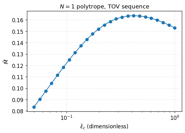
M_max (TOV, N=1)         = 0.1637
e_c at M_max             = 0.4174
4. Sequences I — TOV and the mass-shed limit#
We now build sequences across multiple EOSs. The essential sequences are:
the TOV (static) sequence: gives \(M_{\max}^{\rm TOV}\) — the canonical EOS-discrimination threshold (any EOS with \(M_{\max}^{\rm TOV} < 2\,M_\odot\) is ruled out by the heaviest observed pulsars);
the Kepler (mass-shed) sequence: gives \(\Omega_K(M)\) — the upper envelope of all uniformly rotating equilibria, hence the absolute maximum spin frequency the EOS allows.
# TOV sequence for a few EOSs. Static is essentially free (~1 s for 25 models).
TOV_EOS = ["eosA", "eosC", "eosWS", "eosL", "eosFPS"]
tov = {}
for eos in TOV_EOS:
    tov[eos] = rh.static_sequence(eos, 5e14, 4e15, n=25)

fig, ax = plt.subplots()
for eos in TOV_EOS:
    d = tov[eos]
    ax.plot(d["rho_c"]/1e15, d["M"], label=EOS_LABELS[eos], lw=1.4)
ax.set_xscale("log")
ax.set_xlabel(r"$\varepsilon_c$ (10$^{15}$ g cm$^{-3}$)")
ax.set_ylabel(r"$M$ ($M_\odot$)")
ax.axhline(2.0, color='gray', ls=':', lw=0.8)
ax.text(0.55, 2.03, r"$2\,M_\odot$ pulsar floor", fontsize=8, color='gray')
ax.set_title("TOV mass curves")
ax.legend(loc='lower right', fontsize=8, frameon=False)
plt.tight_layout(); plt.show()

for eos in TOV_EOS:
    d = tov[eos]
    idx = d["M"].idxmax()
    print(f"  {eos:7s}  M_max^TOV = {d.loc[idx,'M']:.3f}  at e_c = {d.loc[idx,'rho_c']:.3e}  R = {d.loc[idx,'R']:.2f} km")
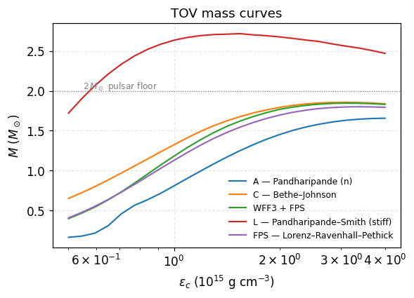
  eosA     M_max^TOV = 1.657  at e_c = 4.000e+15  R = 8.41 km
  eosC     M_max^TOV = 1.857  at e_c = 3.084e+15  R = 9.88 km
  eosWS    M_max^TOV = 1.846  at e_c = 3.084e+15  R = 9.57 km
  eosL     M_max^TOV = 2.716  at e_c = 1.542e+15  R = 13.64 km
  eosFPS   M_max^TOV = 1.801  at e_c = 3.364e+15  R = 9.29 km
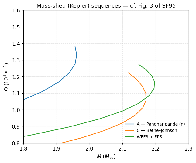
4.1 The mass-shed sequence — reproducing Fig. 3 of Stergioulas & Friedman (1995) (slow)#
This produces \(\Omega\) vs \(M\) along the Kepler limit. The peak is the absolute maximum rotating-mass model for that EOS. Here, we use 15 models per EOS.
# Mass-shed sequence (slow). About 30 s for 15 models per EOS.
MSHED_EOS = ["eosA", "eosC", "eosWS"]   # 3 EOSs ≈ 90 s
mshed = {}
t0 = time.time()
for eos in MSHED_EOS:
    mshed[eos] = rh.kepler_sequence(eos, 8e14, 4e15, n=15)
    print(f"  {eos:6s}: {len(mshed[eos])} models, t = {time.time()-t0:.0f}s")
  eosA  : 15 models, t = 8s
  eosC  : 15 models, t = 16s
  eosWS : 15 models, t = 25s
fig, ax = plt.subplots(figsize=(6.0, 5.0))
for eos in MSHED_EOS:
    d = mshed[eos]
    ax.plot(d["M"], d["Omega"], "-", label=EOS_LABELS[eos], lw=1.5)

ax.set_xlabel(r"$M$ ($M_\odot$)")
ax.set_ylabel(r"$\Omega$ (10$^4$ s$^{-1}$)")
ax.set_title(r"Mass-shed (Kepler) sequences — cf. Fig. 3 of SF95")
ax.set_xlim(1.8, 2.3); ax.set_ylim(0.8, 1.6)
ax.legend(loc='lower right', fontsize=9, frameon=False)
plt.tight_layout(); plt.show()

print("Maximum mass at mass-shed:")
for eos in MSHED_EOS:
    print(f"  {eos:6s}  M_max^rot = {mshed[eos]['M'].max():.3f}  "
          f"(TOV: {tov[eos]['M'].max():.3f},  "
          f"ratio = {mshed[eos]['M'].max()/tov[eos]['M'].max():.3f})")
Maximum mass at mass-shed:
  eosA    M_max^rot = 1.961  (TOV: 1.657,  ratio = 1.184)
  eosC    M_max^rot = 2.171  (TOV: 1.857,  ratio = 1.169)
  eosWS   M_max^rot = 2.196  (TOV: 1.846,  ratio = 1.190)
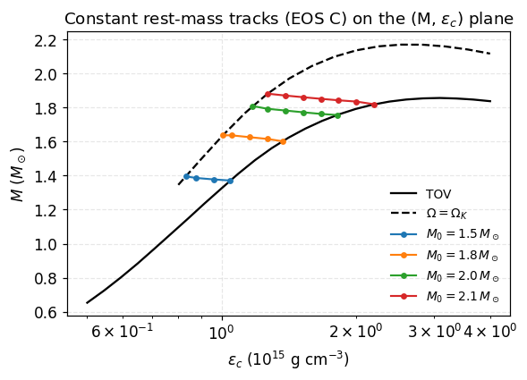
5. Sequences II — constant rest mass and constant angular momentum#
The TOV sequence and the Kepler sequence are the boundaries of the equilibrium region in the \((M, \varepsilon_c)\) plane. The interior of that region is foliated by two natural families of sequences:
Constant rest mass \(M_0\) — a single isolated neutron star evolves along such a track as it loses angular momentum. The endpoint of the spin-down is the TOV model with the same \(M_0\).
Constant angular momentum \(J\) — the orthogonal foliation; \(J\) is conserved on much shorter timescales than \(M_0\) in most astrophysical scenarios.
Together these two families “rule” the surface of equilibria we’ll plot in §6.
# Constant rest-mass tracks for EOS C, using the robust per-model variant
# (some (e_c, M_0) combinations have no equilibrium and would hang the
# native rmass bisection; constant_M0_track_safe skips them cleanly).
M0_vals = [1.5, 1.8, 2.0, 2.1]
m0_tracks = {}
t0 = time.time()
for M0 in M0_vals:
    m0_tracks[M0] = rh.constant_M0_track_safe(
        "eosC", M0=M0, e_min=8.0e14, e_max=2.2e15, n=12,
        per_model_timeout=6.0, include_endpoints=True
    )
    print(f"  M_0 = {M0}: {len(m0_tracks[M0])} models  ({time.time()-t0:.0f} s)")
  M_0 = 1.5: 4 models  (51 s)
  M_0 = 1.8: 5 models  (115 s)
  M_0 = 2.0: 6 models  (191 s)
  M_0 = 2.1: 7 models  (272 s)
fig, ax = plt.subplots()
# TOV envelope
ax.plot(tov["eosC"]["rho_c"]/1e15, tov["eosC"]["M"], "k-", lw=1.5, label="TOV")
# Kepler envelope
ax.plot(mshed["eosC"]["rho_c"]/1e15, mshed["eosC"]["M"], "k--", lw=1.5, label=r"$\Omega = \Omega_K$")
# Constant M_0 tracks
for M0, d in m0_tracks.items():
    d = d.dropna(subset=["M"])
    ax.plot(d["rho_c"]/1e15, d["M"], "o-", ms=3.5, label=f"$M_0 = {M0}\\,M_\\odot$")
ax.set_xscale("log")
ax.set_xlabel(r"$\varepsilon_c$ (10$^{15}$ g cm$^{-3}$)")
ax.set_ylabel(r"$M$ ($M_\odot$)")
ax.set_title("Constant rest-mass tracks (EOS C) on the (M, $\\varepsilon_c$) plane")
ax.legend(loc='lower right', fontsize=9, frameon=False)
plt.tight_layout(); plt.show()
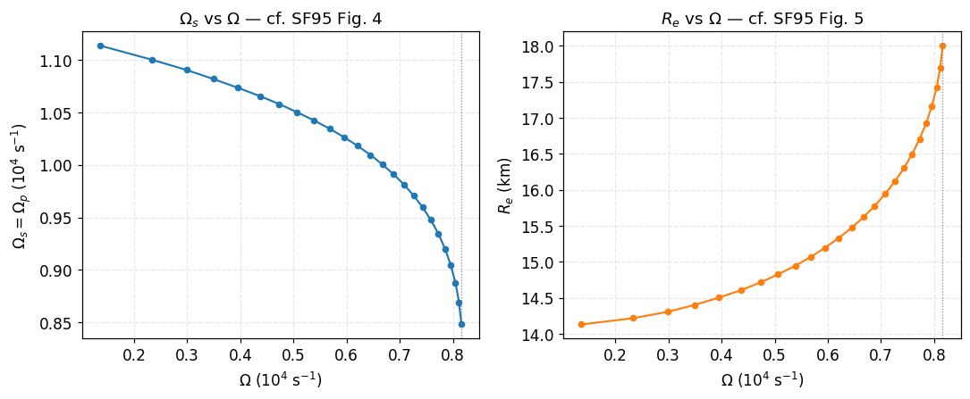
5.1 The \(\Omega_s\) (satellite) frequency near mass-shed — Figs 4–5 of SF95#
The orbital frequency \(\Omega_p\) of a test particle in circular orbit at the equator decreases as \(\Omega\) approaches the mass-shed limit (the surface develops a cusp at the equator). The two derivatives \(|d\Omega_p/d\Omega|\) and \(|dR/d\Omega|\) diverge together.
Along a constant-\(\varepsilon_c\) sequence we can see this directly:
# Walk from low rotation up to the mass-shed limit at fixed e_c.
# We do this by sweeping r_p/r_e for fixed e_c (the 'model' task).
e_c_fixed = 1.21e15   # matches SF95 Fig. 4 (eosL) parameters
r_ratios = np.linspace(0.99, 0.575, 25)
rows = []
for rr in r_ratios:
    try:
        m = rh.run_rns(task="model", eos="eosL", e=e_c_fixed, r=rr)
        rows.append(m.data)
    except Exception:
        pass
df_sweep = pd.DataFrame(rows).dropna(subset=["M"]).sort_values("Omega").reset_index(drop=True)
print(f"{len(df_sweep)} converged models out of {len(r_ratios)}")

fig, axes = plt.subplots(1, 2, figsize=(10, 4.2))
axes[0].plot(df_sweep["Omega"], df_sweep["Omega_p"], "o-", ms=4)
axes[0].set_xlabel(r"$\Omega$ (10$^4$ s$^{-1}$)")
axes[0].set_ylabel(r"$\Omega_s = \Omega_p$ (10$^4$ s$^{-1}$)")
axes[0].set_title(r"$\Omega_s$ vs $\Omega$ — cf. SF95 Fig. 4")

axes[1].plot(df_sweep["Omega"], df_sweep["R_e"], "o-", ms=4, color='C1')
axes[1].set_xlabel(r"$\Omega$ (10$^4$ s$^{-1}$)")
axes[1].set_ylabel(r"$R_e$ (km)")
axes[1].set_title(r"$R_e$ vs $\Omega$ — cf. SF95 Fig. 5")

# Mark mass-shed (last converged model)
mshed_omega = df_sweep["Omega"].iloc[-1]
for ax in axes:
    ax.axvline(mshed_omega, color='gray', ls=':', lw=0.8)
plt.tight_layout(); plt.show()
25 converged models out of 25
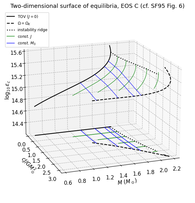
6. The two-dimensional surface of equilibria (slow)#
Eevery uniformly rotating equilibrium of a given EOS lies on a 2-D surface in \((M, J, \varepsilon_c)\), bounded by the TOV curve (\(J=0\)) and the Kepler curve (\(\Omega = \Omega_K\)). We construct that surface by sweeping a family of constant-\(J\) sequences, as shown in Fig. 6 of Stergioulas & Friedman (1995)
The ridge of maximum mass at fixed \(J\) coincides with the onset of (secular) axisymmetric instability (Friedman, Ipser & Sorkin 1988; Cook et al. 1992). Models on the low-\(\varepsilon_c\) side of the ridge are stable against collapse.
# Constant-J ridges for the 2D surface.
# For each J, choose an e_c range that stays inside the equilibrium surface.
# Below e_min: J too large for any equilibrium at that density.
# Above e_max: model becomes axisymmetrically unstable then non-converging.
J_ranges = {
    0.5: (8.0e14, 3.0e15),
    1.0: (1.0e15, 3.0e15),
    1.5: (1.2e15, 3.0e15),
    2.0: (1.4e15, 3.0e15),
    2.5: (1.7e15, 3.0e15),
}
J_tracks = {}
t0 = time.time()
for J, (emin, emax) in J_ranges.items():
    df = rh.constant_J_sequence("eosC", J=J, e_min=emin, e_max=emax, n=10)
    J_tracks[J] = df
    print(f"  J = {J}: {len(df)} models  ({time.time()-t0:.0f} s)")
  J = 0.5: 10 models  (2 s)
  J = 1.0: 10 models  (4 s)
  J = 1.5: 10 models  (7 s)
  J = 2.0: 10 models  (10 s)
  J = 2.5: 10 models  (14 s)
# Surface in (M, J, e_c) -- this is SF95's Fig. 6 for EOS C
from mpl_toolkits.mplot3d import Axes3D  # noqa
from matplotlib.lines import Line2D
fig = plt.figure(figsize=(7, 6))
ax = fig.add_subplot(111, projection='3d')

z_floor = np.log10(1.6e14)

def proj(xs, ys, color, ls="-", lw=0.7):
    ax.plot(xs, ys, z_floor, lw=lw, color=color, ls=ls)

# TOV edge (J = 0)
d0 = tov["eosC"]
ax.plot(d0["M"], np.zeros_like(d0["M"]), np.log10(d0["rho_c"]),
        "k-", lw=1.6, label="TOV ($J=0$)")
proj(d0["M"], np.zeros_like(d0["M"]), color="k", ls="-", lw=1.6)

# Kepler edge
dK = mshed["eosC"]
ax.plot(dK["M"], dK["cJ_GMsun2"], np.log10(dK["rho_c"]),
        "k--", lw=1.6, label=r"$\Omega = \Omega_K$")
proj(dK["M"], dK["cJ_GMsun2"], color="k", ls="--", lw=1.6)

# Constant-J ridges (green)
for J, d in J_tracks.items():
    ax.plot(d["M"], np.full(len(d), J), np.log10(d["rho_c"]),
            "-", lw=1.0, alpha=0.8, color="green")
    proj(d["M"], np.full(len(d), J), color="green", ls="-", lw=1.0)

# Constant-M0 tracks (blue)
for M0, d in m0_tracks.items():
    d = d.dropna(subset=["M", "cJ_GMsun2", "rho_c"]).sort_values("rho_c")
    if len(d) < 2:
        continue
    ax.plot(d["M"], d["cJ_GMsun2"], np.log10(d["rho_c"]),
            "-", lw=1.0, alpha=0.8, color="blue")
    proj(d["M"], d["cJ_GMsun2"], color="blue", ls="-", lw=1.0)

# --- axisymmetric instability ridge ---
def _ridge_point(ec_arr, M_arr):
    """Return (M_max, log10(ec_max)) via central-diff zero-crossing."""
    dM = np.gradient(M_arr, ec_arr)
    k_arr = np.where((dM[:-1] > 0) & (dM[1:] <= 0))[0]
    if len(k_arr) == 0:
        k = np.argmax(M_arr)
        return M_arr[k], np.log10(ec_arr[k])
    k = k_arr[0]
    ec_max = ec_arr[k] - dM[k] * (ec_arr[k+1] - ec_arr[k]) / (dM[k+1] - dM[k])
    M_max  = np.interp(ec_max, ec_arr, M_arr)
    return M_max, np.log10(ec_max)

ridge_pts = []
d0s = tov["eosC"].sort_values("rho_c")
M_r, lec_r = _ridge_point(d0s["rho_c"].values, d0s["M"].values)
ridge_pts.append((M_r, 0.0, lec_r))
for J, d in J_tracks.items():
    ds = d.sort_values("rho_c")
    M_r, lec_r = _ridge_point(ds["rho_c"].values, ds["M"].values)
    ridge_pts.append((M_r, J, lec_r))

ridge_pts.sort(key=lambda x: x[1])
rM, rJ, rlec = zip(*ridge_pts)
ax.plot(rM, rJ, rlec, "k:", lw=1.8, label="instability ridge")
proj(rM, rJ, color="k", ls=":", lw=1.8)

ax.set_xlabel(r"$M$ ($M_\odot$)")
ax.set_ylabel(r"$cJ/GM_\odot^2$")
ax.zaxis.set_rotate_label(False)
ax.set_zlabel(r"$\log_{10}\varepsilon_c$", rotation=90)
ax.set_title("Two-dimensional surface of equilibria, EOS C (cf. SF95 Fig. 6)")
ax.view_init(elev=17, azim=250)
ax.set_ylim(ax.get_ylim()[::-1])
ax.set_zlim(bottom=z_floor)

proxy = [
    Line2D([0], [0], color="green", lw=1.0, label="const. $J$"),
    Line2D([0], [0], color="blue",  lw=1.0, label="const. $M_0$"),
]
ax.legend(handles=ax.get_legend_handles_labels()[0] + proxy,
          labels=ax.get_legend_handles_labels()[1] + ["const. $J$", "const. $M_0$"],
          loc='upper left', fontsize=8)
plt.tight_layout(); plt.show()
6.1 Finding the extremal models#
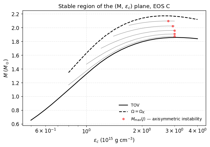
Along each constant-\(J\) track the maximum \(M\) marks the axisymmetric-stability boundary. On the surface as a whole there are four extrema — \(M_{\max}\), \(M_{0,\max}\), \(J_{\max}\), \(\Omega_{\max}\), which, in general, do not coincide.
def _extremum_cd(d):
    """Locate dM/d(rho_c) = 0 via central differences + linear zero-crossing."""
    d = d.sort_values("rho_c").reset_index(drop=True)
    ec = d["rho_c"].values
    M  = d["M"].values
    dM = np.gradient(M, ec)   # central differences at interior points, one-sided at edges
    # find first + -> - sign change (the maximum)
    k_arr = np.where((dM[:-1] > 0) & (dM[1:] <= 0))[0]
    if len(k_arr) == 0:       # no crossing in range -- fall back to discrete argmax
        k = np.argmax(M)
        return ec[k] / 1e15, M[k]
    k = k_arr[0]
    # linear interpolation to sub-grid ec where dM/dec = 0
    ec_max = ec[k] - dM[k] * (ec[k+1] - ec[k]) / (dM[k+1] - dM[k])
    M_max  = np.interp(ec_max, ec, M)
    return ec_max / 1e15, M_max

# Locate extrema across the constant-J ridges and overlay on the (M, e_c) plane
fig, ax = plt.subplots(figsize=(6.5, 4.6))
# Stable region boundary: TOV + Kepler
ax.plot(tov["eosC"]["rho_c"]/1e15, tov["eosC"]["M"], "k-", lw=1.6, label="TOV")
ax.plot(mshed["eosC"]["rho_c"]/1e15, mshed["eosC"]["M"], "k--", lw=1.6,
        label=r"$\Omega = \Omega_K$")

# Constant-J ridges as thin lines, with M_max(J) from derivative zero-crossing
ridge_pts = []
for J, d in J_tracks.items():
    ax.plot(d["rho_c"]/1e15, d["M"], "-", lw=0.8, alpha=0.6, color="0.3")
    ec_max, M_max = _extremum_cd(d)
    ridge_pts.append((ec_max, M_max))
    print(f"  J = {J:.1f}:  e_c(M_max) = {ec_max:.4f} e15,  M_max = {M_max:.5f} M_sun")
xs, ys = zip(*ridge_pts)
ax.plot(xs, ys, "ro", ms=4, alpha=0.5, label="$M_{max}(J)$ — axisymmetric instability")

ax.set_xscale("log")
ax.set_xlabel(r"$\varepsilon_c$ (10$^{15}$ g cm$^{-3}$)")
ax.set_ylabel(r"$M$ ($M_\odot$)")
ax.set_title("Stable region of the (M, $\\varepsilon_c$) plane, EOS C")
ax.legend(loc='lower right', fontsize=9, frameon=False)
plt.tight_layout(); plt.show()
  J = 0.5:  e_c(M_max) = 3.0000 e15,  M_max = 1.87299 M_sun
  J = 1.0:  e_c(M_max) = 3.0000 e15,  M_max = 1.90723 M_sun
  J = 1.5:  e_c(M_max) = 3.0000 e15,  M_max = 1.95889 M_sun
  J = 2.0:  e_c(M_max) = 2.9337 e15,  M_max = 2.02281 M_sun
  J = 2.5:  e_c(M_max) = 2.7784 e15,  M_max = 2.09540 M_sun
7. Astrophysical applications#
Several short worked examples. Each leans on a different output of RNS.
7.1 The ISCO height \(h_+\) — relevance to kHz QPOs#
The innermost stable circular orbit (ISCO) for prograde motion sits at a height \(h_+\) above the equatorial surface. When \(h_+ > 0\) the ISCO is outside the star and an accretion disc truncates there; the orbital frequency at the ISCO is a candidate for the upper kHz QPO frequency observed in LMXBs.
Along a constant-\(M_0\) track, \(h_+\) shrinks with spin: a rapidly spinning star is more oblate and frame-drags more strongly, both of which lower the ISCO.
fig, ax = plt.subplots()
for M0, d in m0_tracks.items():
    d = d.dropna(subset=["Omega", "h_plus"]).sort_values("Omega")
    ax.plot(d["Omega"], d["h_plus"], "o-", ms=4, label=f"$M_0 = {M0}\\,M_\\odot$")
ax.set_xlabel(r"$\Omega$ (10$^4$ s$^{-1}$)")
ax.set_ylabel(r"$h_+$ (km)")
ax.set_title("Prograde ISCO height along constant-$M_0$ tracks (EOS C)")
ax.legend(fontsize=9, frameon=False)
plt.tight_layout(); plt.show()
7.2 Moment of inertia at slow rotation — the double-pulsar test#
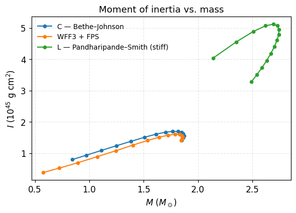
For PSR J0737−3039A in the double pulsar system, \(M = 1.338\,M_\odot\) is known exquisitely well, and the moment of inertia \(I_A\) may be measured to ~10% from spin-orbit coupling within the next decade. Predictions of \(I\) vs \(M\) for different EOSs span a factor of two — a clean future EOS discriminator.
We compute \(I\) along an \(\Omega = \) constant sequence:
# Build I(M) for the EOSs, by sweeping e_c at fixed small Omega.

Omega_value = 0.25     # 10^4 s^-1, i.e. ~400 Hz -> actual rotation rate of PSR J0737−3039A is ~10 times slower
sequence = {}
for eos in ["eosC", "eosWS", "eosL"]:
    d = rh.run_rns(task="omega", eos=eos, Omega=Omega_value,
                   e=6e14, e_max=4e15, n=15).table
    sequence[eos] = d.dropna(subset=["M","I"])

fig, ax = plt.subplots()
for eos, d in sequence.items():
    ax.plot(d["M"], d["I"], "o-", ms=4, label=EOS_LABELS[eos])
ax.set_xlabel(r"$M$ ($M_\odot$)")
ax.set_ylabel(r"$I$ (10$^{45}$ g cm$^2$)")
ax.set_title("Moment of inertia vs. mass")
ax.legend(fontsize=9, frameon=False)
plt.tight_layout(); plt.show()
7.3 Three redshifts vs spin — emission line profiles#
The polar, forward-equatorial, and backward-equatorial redshifts (\(Z_p\), \(Z_f\), \(Z_b\)) bracket the range of redshifts a photon emitted from the surface can suffer. \(Z_f\) can go negative (blueshift) at high spin: the approaching equatorial limb outruns its gravitational redshift.
d = m0_tracks[2.0].sort_values("Omega")
fig, ax = plt.subplots()
ax.plot(d["Omega"], d["Z_p"], "o-", ms=4, label=r"$Z_p$ (polar)")
ax.plot(d["Omega"], d["Z_b"], "s-", ms=4, label=r"$Z_b$ (backward eq.)")
ax.plot(d["Omega"], d["Z_f"], "v-", ms=4, label=r"$Z_f$ (forward eq.)")
ax.axhline(0, color='gray', ls=':', lw=0.8)
ax.set_xlabel(r"$\Omega$ (10$^4$ s$^{-1}$)")
ax.set_ylabel("redshift")
ax.set_title("Surface redshifts along $M_0 = 2\\,M_\\odot$ track, EOS C")
ax.legend(fontsize=9, frameon=False)
plt.tight_layout(); plt.show()
7.4 Frame dragging visualized — using the -p 3 metric printout#
-p 3 prints all four metric potentials (\(\rho, \gamma, \alpha, \omega\)) and the pressure \(P\) on the full computational grid. For a fast-spinning, near-mass-shed model, the dragging potential \(\omega\) is sizable even outside the star — frame dragging is a global feature of the spacetime, not a surface effect.
# Plot omega(s) along the equator from the -p 3 equatorial-slice output.
# Note: -p 3 only outputs the equatorial (mu=0) profile; no polar slice is available.
import subprocess
cmd = [str(rh._binary("std")), "-f", rh._eos_path("eosC"),
       "-t", "kepler", "-e", "2e15", "-p", "3", "-d", "0"]
out = subprocess.run(cmd, capture_output=True, text=True, timeout=60).stdout
grid = rh.parse_metric_grid(out)
print(f"Grid points parsed: {len(grid)}  (equatorial slice, mu=0 throughout)")

# Parse Omega from the 17-token scalar line (index 4: Omega in 10^4 s^-1)
Omega_star = None
for line in out.splitlines():
    toks = line.split()
    if len(toks) == 17:
        try:
            Omega_star = float(toks[4]); break
        except ValueError:
            pass

eq = grid.sort_values("s")
fig, ax = plt.subplots()
ax.plot(eq["s"], eq["omega_pot"], "-", label=r"$\omega(s,\mu{=}0)$")
if Omega_star is not None:
    ax.plot([0, 0.5], [Omega_star, Omega_star], "--", color="C1", lw=1.2,
            label=r"$\Omega$ (uniform rotation)")
ax.set_xlabel(r"$s = r/(r+r_e)$")
ax.set_ylabel(r"$\omega$ (10$^4$ s$^{-1}$)")
ax.set_title("Frame-dragging potential on the equatorial plane, EOS C, e_c = 2\u00d710$^{15}$")
ax.axvline(0.5, color='gray', ls=':', lw=0.8)
ax.text(0.51, eq["omega_pot"].max()*0.9, "surface", fontsize=8, color='gray')
ax.legend(fontsize=9, frameon=False)
plt.tight_layout(); plt.show()
Grid points parsed: 129 (equatorial slice, mu=0 throughout)
8. Where to go next#
This notebook covers the bulk of what RNS does, but several natural extensions deserve their own follow-up:
Modern EOSs — add APR, SLy4, DD2, MPA1, or hybrid quark-matter EOSs. The format is the four-column file described in
eos/EOS.INDEX(ormanual.pdf§3.1); use the bundledHnG.c(compiled here ashng) to convert from \((\varepsilon, P)\) files.Differential rotation — RNS itself assumes uniform rotation, but the same KEH/CST scheme extends naturally (Komatsu, Eriguchi & Hachisu 1989b; Cook–Shapiro–Teukolsky 1992). Hot proto-neutron stars and merger remnants are differentially rotating.
Oscillation modes and stability — RNS provides the equilibrium background; one can then feed it into a perturbation or time evolution code.
Magnetic fields — beyond the perfect-fluid assumption; see Bocquet et al. (1995), Cardall et al. (2001), or the LORENE/Magstar codes.
Strange-quark stars — the EOS for self-bound quark matter (
p = a(\varepsilon - \varepsilon_0)is qualitatively different at the surface (finite density at \(P=0\)); RNS handles them with a small modification.