Surface Regressor Demo

Essential Libraries

import numpy as np
import pandas as pd
import matplotlib.pyplot as plt
from matplotlib.ticker import ScalarFormatter
from matplotlib.ticker import FixedLocator

import seaborn as sns
from mpl_toolkits.mplot3d import Axes3D

import ipywidgets as widgets
from ipywidgets import interactive
from IPython.display import display, Latex

from sklearn.metrics import explained_variance_score, max_error, mean_absolute_error
from sklearn.metrics import mean_squared_error, r2_score, mean_absolute_percentage_error

import UR_utils
from UR_utils import *

import torch
import torch.nn as nn
import torch.optim as optim
from torch.utils.data import DataLoader, TensorDataset
from DNN import Regressor

import os
import re
import time
from zipfile import ZipFile

from scipy import special
from scipy.spatial import ConvexHull,QhullError
from matplotlib.tri import Triangulation, LinearTriInterpolator
from scipy.interpolate import griddata


import warnings
# Disable all warnings
warnings.filterwarnings("ignore")

from matplotlib import rc
rc('mathtext', fontset='cm')

Global variables

device = torch.device('cuda:0' if torch.cuda.is_available() else 'cpu')

if torch.cuda.is_available():
    torch.cuda.set_device(device)


selected_columns = ['cos(theta)', 'R_surf', 'dlogR_dtheta', 'g_surf', 'Rpole_num', 'Req_num', 
                    'Rpol/Req', 'ellipticity', 'eccentricity', 'rho_c', 'r_ratio', 'M', 'M(km)',
                    'Req', 'C', 'K', 'g_0(km^(-1))', 'Ibar', 'f(Hz)', 'f_tilde', 'Jgeom(km^2)',
                    'x', 'sigma', 'T/W', 'Mxf_tilde', 'Rxf_tilde', 'Qbar', 'S3bar', 'EoS']

selected_features = ['|cos(theta)|', 'C', 'sigma', 'eccentricity']

abs_mu_min, abs_mu_max = 0., 1. 
C_min, C_max = 0.0876346858172578, 0.3094541325480277
sigma_min, sigma_max = 0., 0.9612274013913829
eccentricity_min, eccentricity_max = 0., 0.7797886226038347

min_values = np.array([abs_mu_min, C_min, sigma_min, eccentricity_min])
max_values = np.array([abs_mu_max, C_max, sigma_max, eccentricity_max])
feature_scaler = lambda data: (data - min_values) / (max_values - min_values)

N_MU = 521

Read Star Data

def read_zip(file_name, spin, test_percentage=0.2):
    # random seed for 'freezing' randomness
    SEED = 42
    rng = np.random.default_rng(SEED)
    
    # specifying the zip file name
    columns_names = ['cos(theta)', 'R_surf', 'dlogR_dtheta', 'g_surf', 'Rpole_num', 'Req_num', 'Rpol/Req',
                    'ellipticity', 'eccentricity', 'P_c', 'rho_c', 'r_ratio', 'r_e', 'M', 'M(km)',
                    'Req', 'C', 'K', 'g_0(km^(-1))', 'I(kgkm^2)', 'I(km^3)', 'Ibar', 'Z_p', 'Z_b',
                    'Z_f', 'Ω(Hz)', 'f(Hz)', 'f_tilde', 'Jgeom(km^2)', 'x', 'sigma', 'T/W',
                    'Mxf_tilde', 'Rxf_tilde', 'conv_rad', 'conv_plus', 'conv_minus', 'h_plus',
                    'h_minus', 'r_plus', 'r_minus', 'Q(km^3)', 'Qbar', 'S3(km^4)', 'S3bar', 'M4_geom',
                    'M4_asy^GH_geom', 'M4_asy_geom', 'M4_geom_2points', 'M4_geom_3points',
                    'M4_geom_4points', 'S5_geom', 'S5_asy_geom', 'EoS']
    
    minmax_scale = lambda R_mu, Rpole, Req: (R_mu - Rpole) / (Req - Rpole)
    
    df_train, df_test = pd.DataFrame(), pd.DataFrame()
    # opening the zip file in READ mode
    with ZipFile(file_name, 'r') as zip:
        # Pop the folder from the list of stars
        zip.infolist().pop(0)
        
        star_train, star_test = list(), list()
        n_stars = len(zip.infolist())
        n_test_stars = int(n_stars * test_percentage)
        test_indexes = rng.choice(n_stars, n_test_stars, replace=False)
        
        for index, star in enumerate(zip.infolist()):
            star = zip.extract(star)
            df_star = pd.read_csv(star, sep=' ', names=columns_names, skiprows=1)
            
            # Keep stars that have r_ratio >= 0.6
            if df_star['r_ratio'].iloc[0] < 0.6: continue
            repeat_values = df_star.iloc[0].values
            df_star.iloc[1:, 4:] = repeat_values[4:]
            
            # Select only these columns to save memory
            df_star = df_star[selected_columns]
            
            # Output normalization
            if np.all(df_star[spin] == 0.0):
                # Avoid zero division for the static case
                df_star['R_scaled'] = df_star['R_surf']
            else:
                # Min max scaling at star level
                df_star['R_scaled'] = minmax_scale(df_star['R_surf'], df_star['Rpole_num'].iloc[0], df_star['Req_num'].iloc[0])
            
            if index in test_indexes:
                star_test.append(df_star)
            else:
                star_train.append(df_star)
                
        # Concatenate the dataframes for training and test datasets
        if star_train: df_train = pd.concat(star_train, ignore_index=True)
        if star_test: df_test = pd.concat(star_test, ignore_index=True)
        
    return df_train, df_test

def load_stars(df, batch_size=4096, shuffle=True):
    df_target = df['R_scaled']
    
    # Z_2 Symmetry constrain
    df['|cos(theta)|'] = np.abs(df['cos(theta)'])

    np_features = df[selected_features].to_numpy()    
    np_targets = df_target.to_numpy()
    np_targets = np.reshape(np_targets, (np_targets.shape[0], 1))
    
    tr_features = torch.Tensor(feature_scaler(np_features))
    input_dimension = tr_features.shape[1]
    
    tr_targets = torch.Tensor(np_targets)
    final_dataset = TensorDataset(tr_features, tr_targets)

    dataloader = DataLoader(final_dataset, batch_size=batch_size, shuffle=shuffle, num_workers=1, pin_memory=True)

    return dataloader, input_dimension, np_features, np_targets

def Surface_plot(df, x,y,w, z, xlabel,ylabel,wlabel,zlabel, view2, n_col,
                         border_axes, X,Y,W, Z, l_w):
    
    fig = plt.figure(figsize=(20 ,16)) 
    labels_text_size = 40
    ax = fig.add_subplot(111, projection='3d')

    dot_size = 40
    font_size = 40
    label_pad = 40
    label_size = 30

    
    #######################################################################################################
    mu_values = [0.000,0.45769231,0.78461538,1.000]
    colors = ['green', 'pink', 'cyan', 'purple']
    
    for i in range(0,len(mu_values)):
        scatter = ax.scatter(df[df['mu']==mu_values[i]][x].to_numpy(), df[df['mu']==mu_values[i]][y].to_numpy(),df[df['mu']==mu_values[i]][z].to_numpy(),
                   c = df[df['mu']==mu_values[i]][w].to_numpy(), s = dot_size, cmap='coolwarm', marker='o', alpha = 0.8)    


        triang = Triangulation(df[df['mu']==mu_values[i]][x].to_numpy(), df[df['mu']==mu_values[i]][y].to_numpy())
        interpolator = LinearTriInterpolator(triang, df[df['mu']==mu_values[i]][z].to_numpy())
        grid_x, grid_y = np.mgrid[0.0901155694351282:0.3062042574717896:500j, 0.0329041860812303:0.9416722276120412:500j]
        grid_z = interpolator(grid_x, grid_y)
        
        
        
        ax.plot_surface(grid_x, grid_y, grid_z, color = colors[i], alpha = 0.8, label = f'Interpolated surface with $\mu_\star$ = {np.round(mu_values[i],3)}', zorder = 5)

   
    # Add colorbar
    cbar = plt.colorbar(scatter,  shrink=0.5)
    cbar.set_label(wlabel, fontsize=font_size, rotation=0)
    cbar.ax.tick_params(labelsize=23)


    
    ax.view_init(30, view2)   
    ax.set_xlabel(xlabel, fontsize=font_size,labelpad=label_pad) 
    ax.set_ylabel(ylabel, fontsize=font_size,labelpad=label_pad)
    
    ax.zaxis.set_rotate_label(False) 
    ax.set_zlabel(zlabel, fontsize=font_size,labelpad=label_pad,rotation = 90)  
    #ax.yaxis._axinfo['label']['space_factor'] = 3.0   

    ax.zaxis.labelpad = 25
    
    ax.xaxis.set_tick_params(labelsize=label_size)
    ax.yaxis.set_tick_params(labelsize=label_size)
    ax.zaxis.set_tick_params(labelsize=label_size)
    
    for axis in [ax.xaxis, ax.yaxis, ax.zaxis]:
        axis.line.set_linewidth(3)
    
    ax.grid(False)


    leg = plt.legend(loc="upper right",ncol=n_col, borderaxespad=border_axes, prop={'size': 20}, shadow=True, fontsize="large")    #,bbox_to_anchor=(1,1)
    leg.get_frame().set_linewidth(3.0)
    leg.get_frame().set_edgecolor('black')
    
    plt.tight_layout()
    
    plt.show()

Evaluation: Statistical evaluation measures

Evaluation of the total Regression ANN model performance to the whole NSs Dataset [test set]

df_eval_dataset = pd.read_csv('./Experimental Results/Surface/dataset_measures.csv')
df_eval_dataset

	explained_variance	max_error	mean_absolute_error	mean_squared_error	r2_score	mean_absolute_percentage_error	eval_eos_type	eval_eos_name
0	0.999997	0.033331	0.001149	0.000006	0.999997	0.00009	NaN	NaN

Evaluation of the trained ANN model to the whole NS’s data (per EOS level) [test dataset]

df_eval_eos = pd.read_csv('./Experimental Results/Surface/EOS_measures.csv')
df_eval_eos = df_eval_eos.sort_values(by = ['eval_eos_type', 'eval_eos_name'])
df_eval_eos.reset_index(drop = True, inplace = True)
df_eval_eos[0:30]

	explained_variance	max_error	mean_absolute_error	mean_squared_error	r2_score	mean_absolute_percentage_error	eval_eos_type	eval_eos_name
0	0.999999	0.011260	0.000682	0.000002	0.999999	0.000057	Hadronic	BL_2018
1	0.999997	0.014408	0.000963	0.000004	0.999997	0.000074	Hadronic	BSK22
2	0.999997	0.020043	0.000908	0.000004	0.999997	0.000071	Hadronic	BSK24
3	0.999993	0.024129	0.001499	0.000010	0.999991	0.000119	Hadronic	BSK25
4	0.999997	0.017419	0.001138	0.000004	0.999996	0.000097	Hadronic	BSK26
5	0.999997	0.014428	0.000854	0.000003	0.999997	0.000072	Hadronic	D1M*
6	0.999991	0.017989	0.002098	0.000012	0.999991	0.000163	Hadronic	DDHδ
7	0.999995	0.021116	0.001338	0.000007	0.999994	0.000097	Hadronic	DS(CMF)-2
8	0.999998	0.014938	0.000863	0.000002	0.999998	0.000064	Hadronic	DS(CMF)-4
9	0.999999	0.016749	0.000649	0.000002	0.999999	0.000049	Hadronic	DS(CMF)-6
10	0.999999	0.015427	0.000582	0.000002	0.999999	0.000044	Hadronic	DS(CMF)-8
11	0.999996	0.019850	0.001592	0.000008	0.999994	0.000121	Hadronic	FSU2R
12	0.999998	0.015126	0.001054	0.000004	0.999997	0.000094	Hadronic	KDE0v
13	0.999999	0.009924	0.000599	0.000001	0.999999	0.000052	Hadronic	KDE0v1
14	0.999992	0.027231	0.001965	0.000017	0.999990	0.000148	Hadronic	MTVTC
15	0.999997	0.019523	0.000979	0.000005	0.999996	0.000074	Hadronic	PCSB1
16	0.999999	0.010655	0.000636	0.000002	0.999999	0.000050	Hadronic	PCSB2
17	0.999994	0.019471	0.002008	0.000011	0.999991	0.000166	Hadronic	QMC-RMF2
18	0.999994	0.016572	0.001750	0.000010	0.999991	0.000143	Hadronic	QMC-RMF3
19	0.999993	0.019951	0.001824	0.000011	0.999991	0.000143	Hadronic	QMC-RMF4
20	0.999996	0.024136	0.001288	0.000007	0.999995	0.000098	Hadronic	Rs
21	0.999998	0.014135	0.001130	0.000005	0.999997	0.000084	Hadronic	SK255
22	0.999998	0.014136	0.001042	0.000004	0.999998	0.000077	Hadronic	SK272
23	0.999997	0.023211	0.001481	0.000008	0.999996	0.000109	Hadronic	SKI2
24	0.999998	0.017293	0.001009	0.000004	0.999997	0.000074	Hadronic	SKI3
25	0.999995	0.014670	0.001370	0.000007	0.999995	0.000109	Hadronic	SKI4
26	0.999994	0.024094	0.001921	0.000014	0.999992	0.000136	Hadronic	SKI5
27	0.999997	0.014977	0.001034	0.000004	0.999997	0.000083	Hadronic	SKI6
28	0.999997	0.014723	0.000920	0.000004	0.999997	0.000070	Hadronic	SKa
29	0.999990	0.026229	0.001728	0.000012	0.999989	0.000140	Hadronic	SKb

Evaluation measures for the trained ANN model to the star level [NSs at test dataset]

#note: follow the ./Experimental Results/Surface/ path and unzip the perc_error_star_level.zip file
df = pd.read_csv('./Experimental Results/Surface/perc_error_star_level.csv')

df['min_max'] = (df['R_surf'] - df['Rpole'])/(df['Req'] - df['Rpole'])

C_min = df[df['sigma'] != 0]['C'].min(); C_max = df[df['sigma'] != 0]['C'].max();
sigma_min = df[df['sigma'] != 0]['sigma'].min(); sigma_max = df[df['sigma'] != 0]['sigma'].max()

df_new = df[df['sigma'] !=0].copy()
df_new.reset_index(drop=True, inplace=True)

R_min_max = (df_new['R_surf'] - df_new['Rpole'])/(df_new['Req'] - df_new['Rpole'])
mu_var = df_new['mu']
e_var = df_new['eccentricity']
z_1 = np.abs(df_new['percentange_error'])
C_var = df_new['C']
sigma_var = df_new['sigma']

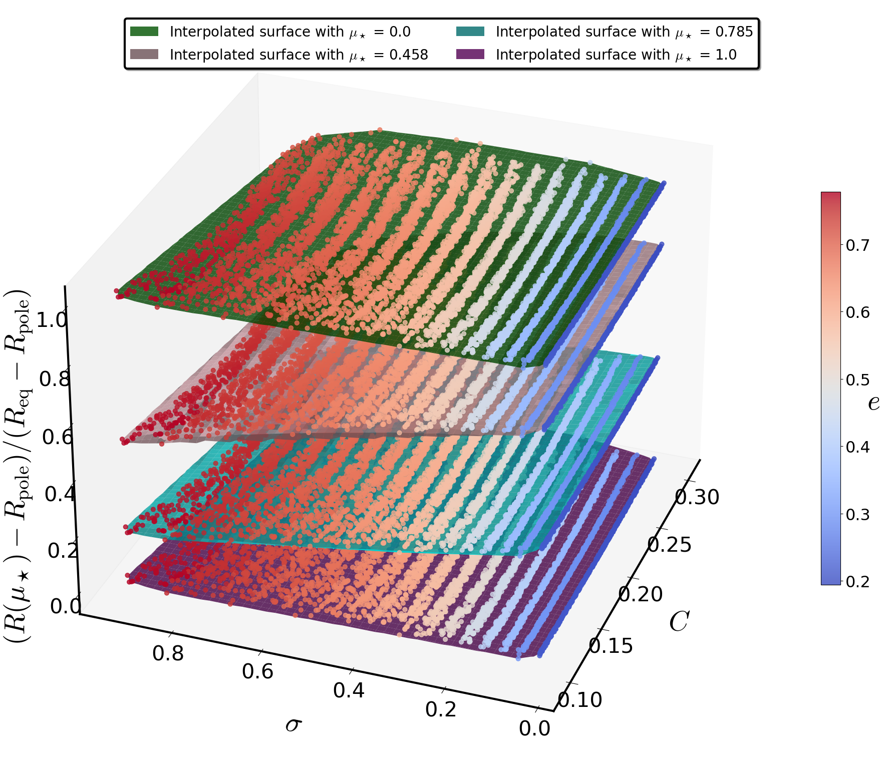
Universal description for fixed \(\mu\) values

x = 'C'; y = 'sigma'; w = 'eccentricity' ;z = 'min_max' ; z_model = '';

Surface_plot(df_new, x,y,w,z, xlabel=r'$C$',ylabel='$\sigma$',
                     wlabel = r'$e$',zlabel=r'$(R(\mu_\star) - R_{\mathrm{pole}})/(R_{\mathrm{eq}} - R_{\mathrm{pole}})$', 
                     view2=200, n_col=2, border_axes=1, X=None,Y=None,W = None,Z=None, l_w=1.5)

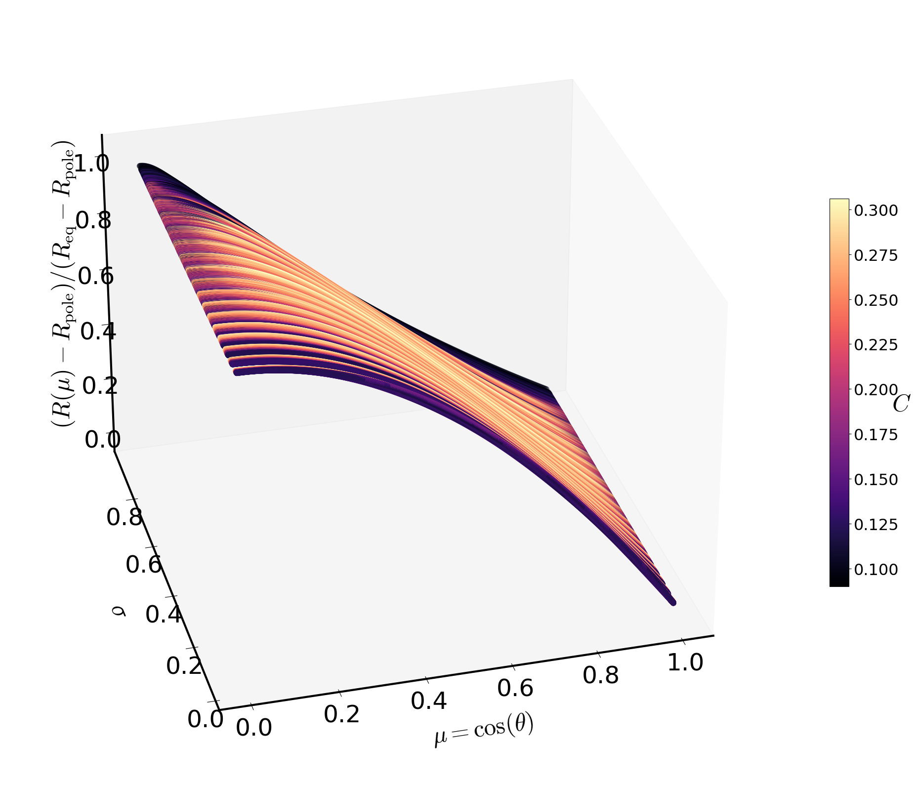
Universal description for each \(\mu\) value

fig = plt.figure(figsize=(20, 16))
labels_text_size = 40
ax = fig.add_subplot(111, projection='3d')
dot_size = 60
font_size = 35
label_pad = 35
label_size = 35

scatter = ax.scatter(mu_var, sigma_var, R_min_max, c=C_var, cmap='magma', s=60)  # q affects color and size

cbar = plt.colorbar(scatter,  shrink=0.5, )
cbar.set_label(r'$C$', fontsize=font_size,rotation=0)
cbar.ax.tick_params(labelsize=23)

ax.view_init(30, 255)   
    

ax.set_xlabel(r'$\mu = \cos (\theta)$', fontsize=font_size,labelpad=label_pad) 

ax.set_ylabel(r'$\sigma$', fontsize=font_size,labelpad=label_pad) 

ax.zaxis.set_rotate_label(False) 
ax.set_zlabel(r'$(R(\mu) - R_{\mathrm{pole}})/(R_{\mathrm{eq}} - R_{\mathrm{pole}})$', fontsize=font_size,labelpad=label_pad,rotation = 90) 

ax.zaxis.labelpad = 25
    
ax.xaxis.set_tick_params(labelsize=label_size)
ax.yaxis.set_tick_params(labelsize=label_size)
ax.zaxis.set_tick_params(labelsize=label_size)
    
for axis in [ax.xaxis, ax.yaxis, ax.zaxis]:
    axis.line.set_linewidth(3)
    
ax.grid(False)
    
plt.tight_layout()

plt.show()

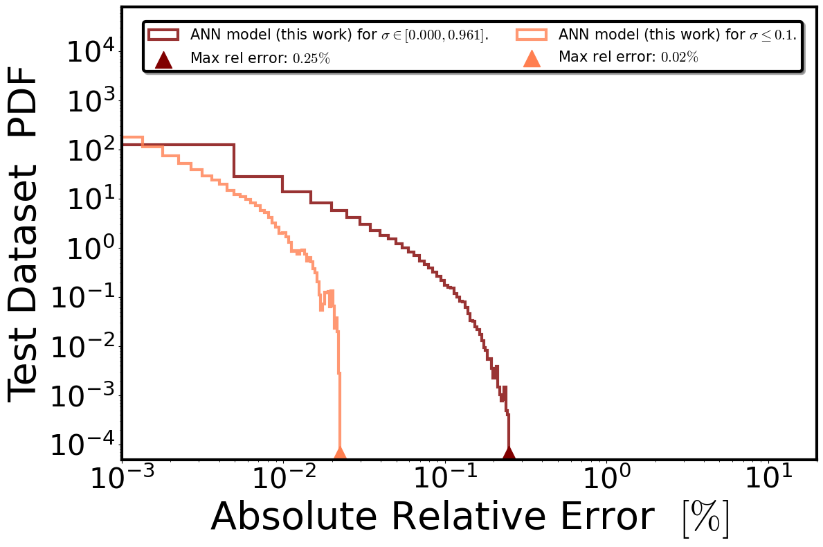
Percentage error histogram in the test set for the suggested ANN model optimal weights

fig, ax = plt.subplots(figsize=(12, 8))
labels_text_size = 40
plt.xticks(fontsize=30)
plt.yticks(fontsize=30)

xlabel = r'Absolute Relative Error  $[\%]$'
ylabel = r'Test Dataset  PDF'

plt.xlabel(xlabel, size=labels_text_size)
plt.ylabel(ylabel, size=labels_text_size)

bins = 50
alpha = 0.8
# Histogram of errors aoociated with the proposed ANN Regression Model for at all sigma
y_reg_errors = abs(df['percentange_error']).hist(
                    density = True,
                    lw = 3,
                    bins=bins,
                    edgecolor='maroon',
                    histtype='step',
                    zorder=1, alpha=alpha, 
                    label='ANN model (this work) for $\sigma \in [0.000, 0.961]$.', color='maroon').autoscale(enable=True, axis='both', tight=True)

# Vertical line for the proposed ANN Regression Model
vertical_lines = [abs(df['percentange_error']).max(), None]
plt.scatter(vertical_lines[0], 0.65e-4, color='maroon', marker='^', s=300, zorder=2, label=f"Max rel error: ${np.round(abs(df['percentange_error']).max(),2)} \%$")  # Star marker

# Histogram of errors aoociated with the proposed ANN Regression Model for sigma <= 0.1
y_reg_errors_2 = abs(df[df['sigma']<=0.1]['percentange_error']).hist(
                    density = True,
                    lw = 3,
                    bins=bins,
                    edgecolor='coral',
                    histtype='step',
                    zorder=1, alpha=alpha, 
                    label='ANN model (this work) for $\sigma \leq 0.1$.', color='coral').autoscale(enable=True, axis='both', tight=True)

# Vertical line for the proposed ANN Regression Model evaluated at sigma <=1
vertical_lines = [abs(df[df['sigma']<=0.1]['percentange_error']).max(), None]

plt.scatter(vertical_lines[0], 0.65e-4, color='coral', marker='^', s=300, zorder=2, label=f"Max rel error: ${np.round(abs(df[df['sigma']<=0.1]['percentange_error']).max(),2)} \%$")  # Star marker

# Customize plot appearance
for axis in ['top', 'bottom', 'left', 'right']:
    ax.spines[axis].set_linewidth(3.0)

# Set logarithmic scale 
plt.xscale('log')
plt.yscale('log')

# Adjust x,y-axis limits (optional, based on log scale)
plt.xlim(0.1e-2,20)
plt.ylim(5e-5,80000)

# Grid, legend, and layout
plt.grid(False)
leg = plt.legend(loc="upper right", ncol=2, borderaxespad=1, prop={'size': 15.},  shadow=True, fontsize="large")
leg.get_frame().set_linewidth(3.0)
leg.get_frame().set_edgecolor('black')
plt.tight_layout()
plt.show()

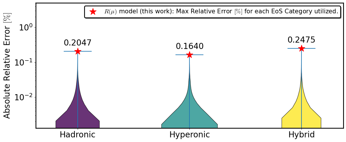
Distribution of absolute Relative Errors for each EoS category in the test set

eos_categories = ['Hadronic', 'Hyperonic', 'Hybrid']

EoS_categories_violin_plots(
    eos_categories = eos_categories, 
    df = df, 
    eval_metric = 'percentange_error', 
    color_map = 'viridis', 
    label = r'$R(\mu)$ model (this work): Max Relative Error $[\%]$ for each EoS Category utilized.', 
    scale = 'log',
    y_max = 5,
    y_label = r"Absolute Relative Error $[\%]$")

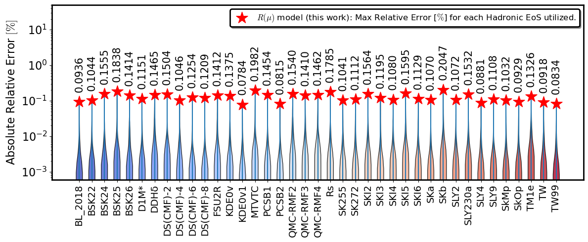
Distribution of absolute Relative Errors for Hadronic EoSs in the test set

eos_names = [ 'BL_2018', 'BSK22', 'BSK24', 'BSK25', 'BSK26', 'D1M*', 'DDHδ','DS(CMF)-2', 'DS(CMF)-4', 'DS(CMF)-6', 'DS(CMF)-8', 'FSU2R',
       'KDE0v', 'KDE0v1', 'MTVTC', 'PCSB1', 'PCSB2', 'QMC-RMF2','QMC-RMF3', 'QMC-RMF4', 'Rs', 'SK255', 'SK272', 'SKI2', 'SKI3',
       'SKI4', 'SKI5', 'SKI6', 'SKa', 'SKb', 'SLY2', 'SLY230a', 'SLY4', 'SLY9', 'SkMp', 'SkOp', 'TM1e', 'TW', 'TW99']


EoS_class_violin_plots(eos_names = eos_names, 
                 df = df, 
                 eval_metric = 'percentange_error', 
                 eos_class = 'Hadronic EoSs', 
                 color_map = 'coolwarm', 
                 label = r'$R(\mu)$ model (this work): Max Relative Error [$\%$] for each Hadronic EoS utilized.', 
                 scale = 'log',      
                 y_max = 50, 
                 y_label = r"Absolute Relative Error $[\%]$")

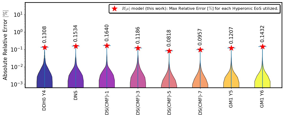
Distribution of absolute Relative Errors for Hyperonic EoSs in the test set

eos_names = [ 'DDHδ Υ4', 'DNS', 'DS(CMF)-1', 'DS(CMF)-3', 'DS(CMF)-5','DS(CMF)-7', 'GM1 Y5', 'GM1 Y6']

EoS_class_violin_plots(eos_names = eos_names, 
                 df = df, 
                 eval_metric = 'percentange_error', 
                 eos_class = 'Hyperonic EoSs', 
                 color_map = 'plasma', 
                 label = r'$R(\mu)$ model (this work): Max Relative Error [$\%$] for each Hyperonic EoS utilized.', 
                 scale = 'log',      
                 y_max = 50, 
                 y_label = r"Absolute Relative Error $[\%]$")

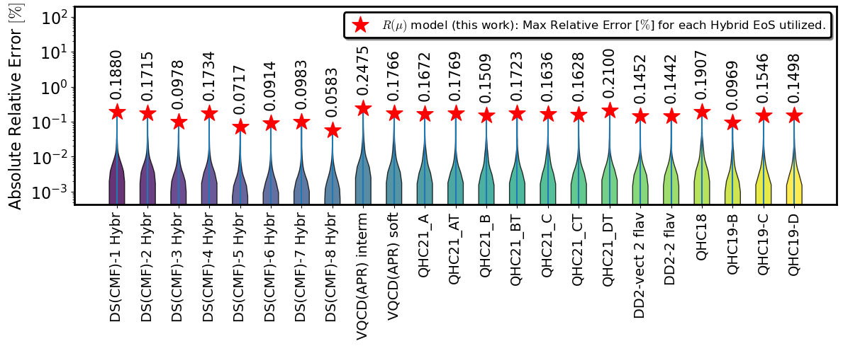
Distribution of absolute Relative Errors for Hybrid EoSs in the test set

eos_names = ['DS(CMF)-1 Hybrid', 'DS(CMF)-2 Hybrid', 'DS(CMF)-3 Hybrid','DS(CMF)-4 Hybrid', 'DS(CMF)-5 Hybrid', 'DS(CMF)-6 Hybrid',
       'DS(CMF)-7 Hybrid', 'DS(CMF)-8 Hybrid','JJ(VQCD(APR)), intermediate', 'JJ(VQCD(APR)), soft','KBH(QHC21_A)', 'KBH(QHC21_AT)', 'KBH(QHC21_B)', 'KBH(QHC21_BT)',
       'KBH(QHC21_C)', 'KBH(QHC21_CT)', 'KBH(QHC21_DT)','OOS(DD2)-vect interaction 2 flavors', 'OOS(DD2-FRG)-2 flavors',
       'QHC18', 'QHC19-B', 'QHC19-C', 'QHC19-D']

EoS_class_violin_plots(eos_names = eos_names, 
                 df = df, 
                 eval_metric = 'percentange_error', 
                 eos_class = 'Hybrid EoSs', 
                 color_map = 'viridis', 
                 label = r'$R(\mu)$ model (this work): Max Relative Error [$\%$] for each Hybrid EoS utilized.',
                 scale = 'log',      
                 y_max = 200, 
                 y_label = r"Absolute Relative Error $[\%]$")

ANN Regression Model for star’s surface: Evaluation on singular EOS

# Choose the case/EoS of your preference
# In this demo we provide indicatively for demonstration 3 EoS: 1 per star's category investigated

# Hadronic case
#file_name = './Surface models for Hadronic EOS/SLY4/'

# Hyperonic case
#file_name = './Surface models for Hyperonic EOS/DNS/'

# Hybrid case
file_name = './Surface models for Hybrid EOS/KBH(QHC21_AT)/'

spin = 'sigma' 
test_percentage = 0.2

rotational_path = os.path.join(file_name, 'rotational_models.zip')
static_path = os.path.join(file_name, 'static_models.zip')

df_rot_train, df_rot_test = read_zip(rotational_path, spin=spin, test_percentage=test_percentage)
df_stat_train, df_stat_test = read_zip(static_path, spin=spin, test_percentage=test_percentage)

df_train = pd.concat([df_rot_train, df_stat_train], ignore_index=True)
df_test = pd.concat([df_rot_test, df_stat_test], ignore_index=True)

# Free the memory space
del df_rot_train, df_rot_test, df_stat_train, df_stat_test

Load the Regression Model optimal weights to estimate star’s surface

batch_size = 4096
model_path = './Model/Surface/Surface-model.pth'

dataloader_tr, input_dimension, np_features_tr, np_targets_tr = load_stars(df_train, batch_size=batch_size)
dataloader_ts, _, np_features_ts, np_targets_ts = load_stars(df_test, batch_size=batch_size)

regressor = Regressor(input_dimension=input_dimension, feature_scaler=feature_scaler).to(device)
regressor.set_device(device)
regressor.load_state_dict(torch.load(model_path, map_location=torch.device(device)))
regressor.eval()

Regressor(
  (MLP): Sequential(
    (0): Linear(in_features=4, out_features=200, bias=True)
    (1): LeakyReLU(negative_slope=0.1, inplace=True)
    (2): Linear(in_features=200, out_features=100, bias=True)
    (3): LeakyReLU(negative_slope=0.1, inplace=True)
    (4): Linear(in_features=100, out_features=50, bias=True)
    (5): LeakyReLU(negative_slope=0.1, inplace=True)
    (6): Linear(in_features=50, out_features=25, bias=True)
    (7): LeakyReLU(negative_slope=0.1, inplace=True)
    (8): Linear(in_features=25, out_features=10, bias=True)
    (9): LeakyReLU(negative_slope=0.1, inplace=True)
    (10): Linear(in_features=10, out_features=1, bias=True)
    (11): Sigmoid()
  )
)

Plot functions associated with residual and percentage errors

def plot_residuals(residual_error, percentage_error):
    witdh, height = 16, 6
    fontsize = 20
    labelsize = 15
    lw = 5
    
    fig, ax = plt.subplots(1, 2, figsize=(witdh, height))
    # Residual error subplot 
    ax[0].plot(residual_error, lw=lw)
    ax[0].set_xlabel(r'Datapoints', fontsize=fontsize)
    ax[0].set_ylabel(r'Residual', fontsize=fontsize)
    ax[0].tick_params(axis='both', which='both', labelsize=labelsize)

    # Percentage error subplot 
    ax[1].plot(percentage_error, lw=lw)
    ax[1].set_xlabel(r'Datapoints', fontsize=fontsize)
    ax[1].set_ylabel(r'Percentage Error$\ [\%]$', fontsize=fontsize)
    ax[1].tick_params(axis='both', which='both', labelsize=labelsize)

    plt.tight_layout()
    plt.show()
    
    fig, ax = plt.subplots(1, 2, figsize=(16, 6))
    fontsize = 20
    labelsize = 15
    lw = 5

    # Residual errors histogram
    ax[0].hist(residual_error, lw=lw)
    ax[0].set_ylabel(r'Data points', fontsize=fontsize)
    ax[0].set_xlabel(r'Residual', fontsize=fontsize)
    ax[0].tick_params(axis='both', which='both', labelsize=labelsize)

    # Percentage errors histogram
    ax[1].hist(percentage_error, lw=lw)
    ax[1].set_ylabel(r'Data points', fontsize=fontsize)
    ax[1].set_xlabel(r'Percentage Error $[\%]$', fontsize=fontsize)
    ax[1].tick_params(axis='both', which='both', labelsize=labelsize)

    plt.tight_layout()
    plt.show()

def plot_surface(mu, model_estimation, real_targets, C, sigma):
    witdh, height = 10, 6
    fontsize = 20
    labelsize = 20
    lw = 5

    fig, ax = plt.subplots(figsize=(witdh, height))
    ax.plot(mu, model_estimation, lw=lw, c='maroon', label='ANN model (this work)')
    ax.scatter(mu, real_targets, c='black', s=20, marker='o', label='Numerical Data')
    
    plt.ylim(real_targets.min()-0.5, real_targets.max()+0.5)
    plt.xlabel(r'$\mu = \cos(\theta)$', fontsize=fontsize)
    plt.ylabel(r'$R(\mu) \ [\mathrm{km}]$', fontsize=fontsize)
    plt.title(f'NS model with C={round(C,3)}, $\sigma$ = {round(sigma,3)}')
    plt.legend(loc='best', prop={'size':fontsize}, shadow=True, fontsize='large')
    ax.tick_params(axis='both', which='both', labelsize=labelsize)

    leg = plt.legend(loc="upper right", ncol=2, borderaxespad=1, prop={'size': 15.},  shadow=True, fontsize="large")
    leg.get_frame().set_linewidth(3.0)
    leg.get_frame().set_edgecolor('black')
    plt.tight_layout()
    plt.show()
    

Universal relations suggested in this work for the parameters \(e = \sqrt{1-(R_p/R_e)^2}\) and \(\mathcal{R} \equiv R_p/R_e\)

#def eccentricity(C, sigma):
#    return (
#        -99.173162625833 * C**5 +68.055729822908 * C**4 * sigma + 137.191420602024 * C**4 +12.9349885313244 * C**3 * sigma**2 -
#        57.474308297241 * C**3 * sigma -67.7948794729071 * C**3 -9.03315944594535 * C**2 * sigma**3 + 8.08346062523145 * C**2 * sigma**2 +
#        9.19713339469957 * C**2 * sigma + 14.9006458417145 * C**2 + 4.84885244516378 * C * sigma**4 -
#        6.44626099699536 * C * sigma**3 +2.75499036217858 * C * sigma**2 -
#        1.3329369261108 * C * sigma - 1.52533604289959 * C + 4.71450473450295 * sigma**5 -
#        13.8547513636472 * sigma**4 + 15.4712200610891 * sigma**3 - 8.71280504897915 * sigma**2 +
#        3.0422989983075 * sigma + 0.182560763719325
#    )


#def R_pole(R_e, C, sigma):
#    return (
#        R_e*(-45.3015234274801 * C**4 - 7.52466249012259 * C**3 * sigma
#        + 36.1318805958812 * C**3 - 2.50668582910242 * C**2 * sigma**2
#        + 8.66838156199219 * C**2 * sigma - 10.4561101976216 * C**2
#        + 0.527775373801867 * C * sigma**3 - 0.226904263928412 * C * sigma**2
#        - 1.45892092679705 * C * sigma + 1.29663161750561 * C + 0.196118434593753 * sigma**4
#        - 0.440968195037673 * sigma**3 + 0.544639042230603 * sigma**2 - 0.617710700567153 * sigma
#        + 0.942328028476575)
#    )

Select NS model for surface illustration and residuals visualization

# Select Set (Train/Test)
is_train = True # True or False

# Select your favorite Star
star_index = 110

# Do not change
low = star_index * N_MU
high = (star_index + 1) * N_MU

select_set = lambda is_train, df_train, df_test: df_train if is_train else df_test
select_features = lambda is_train, np_features_tr, np_features_ts: np_features_tr if is_train else np_features_ts
select_targets = lambda is_train, np_targets_tr, np_targets_ts: np_targets_tr if is_train else np_targets_ts
    
# Select Set (Train/Test)
df_set = select_set(is_train, df_train, df_test)
features = select_features(is_train, np_features_tr, np_features_ts)
targets = select_targets(is_train, np_targets_tr, np_targets_ts)


# estimate the star's surface using the ANN model
estimation = regressor.predict(features[low:high])
maxmin_diff = df_set['Req_num'].iloc[low] - df_set['Rpole_num'].iloc[low]
min_ = df_set['Rpole_num'].iloc[low]

# Using results from the suggested universal relations:
#maxmin_diff = df_set['Req_num'].iloc[low] -  R_pole(df_set['Req_num'].iloc[low], df_set['C'].iloc[low], df_set['sigma'].iloc[low])
#min_ = R_pole(df_set['Req_num'].iloc[low], df_set['C'].iloc[low], df_set['sigma'].iloc[low])
###################################################################################################################################
# Static case
if np.all(df_set['sigma'].iloc[low:high] == 0):
    model_estimation = estimation * df_set['Req_num'].iloc[low]
    real_targets = targets[low:high] * df_set['Req_num'].iloc[low]
# Rotational case
else:
    model_estimation = estimation * (maxmin_diff) + min_ 
    real_targets = targets[low:high] * (maxmin_diff) + min_
    
mu = df_set['cos(theta)'].iloc[low:high]

Residual and Percentage error representations

residual_error = model_estimation - real_targets
percentage_error = (residual_error / real_targets) * 100

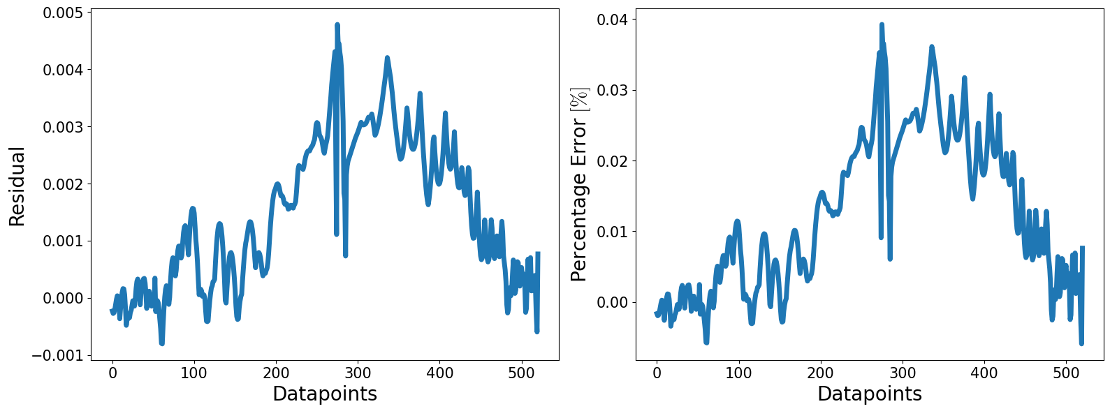
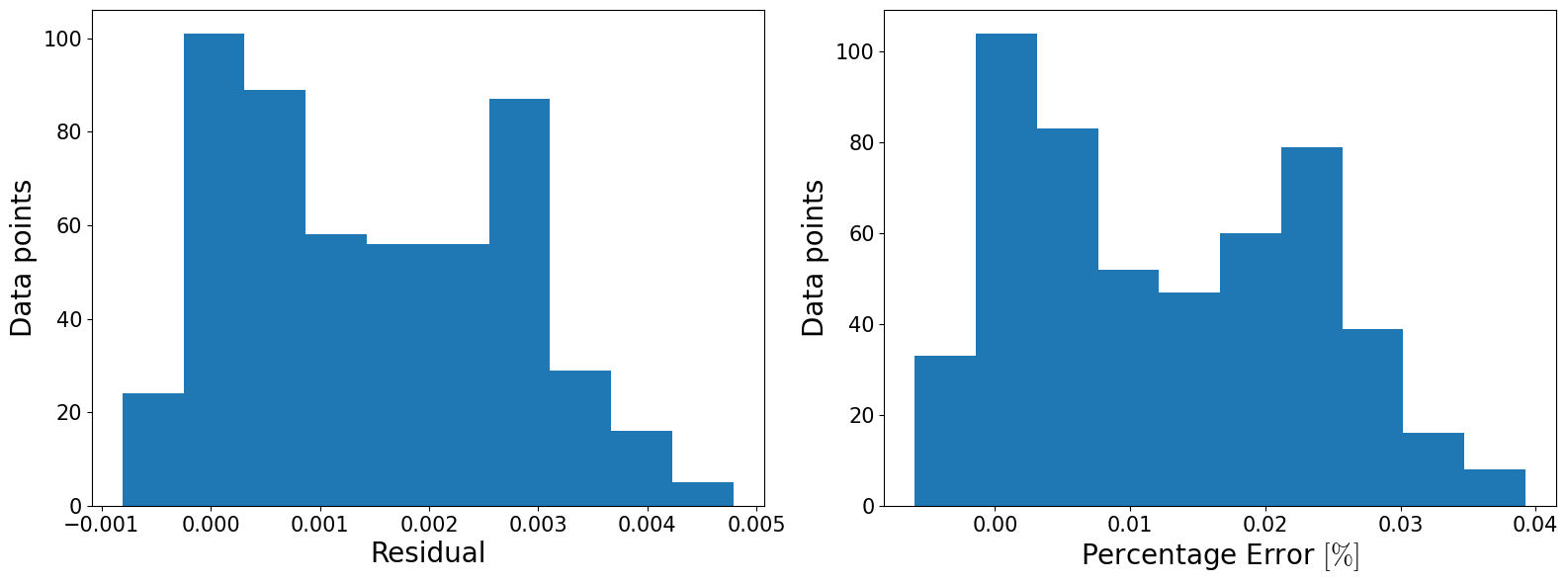
Error distributions a singular NS configuration

plot_residuals(residual_error, percentage_error)

Surface \(R(\mu)\) for an indicative NS configuration

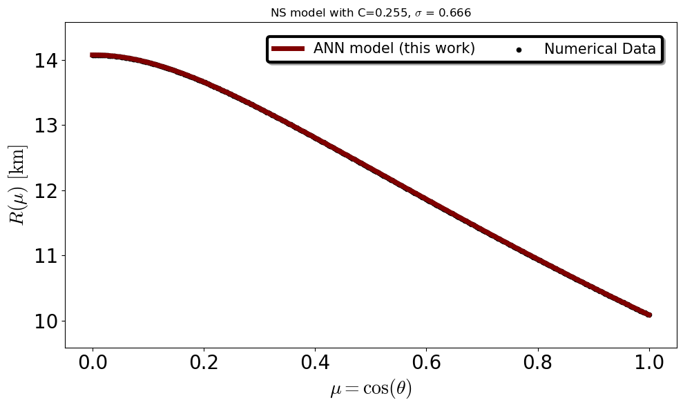
plot_surface(mu, model_estimation, real_targets, df_set['C'].iloc[star_index * N_MU], df_set['sigma'].iloc[star_index * N_MU])

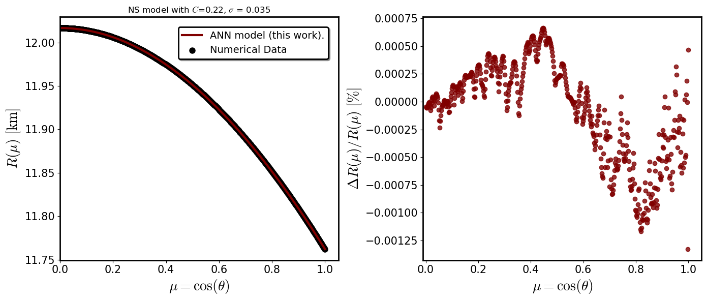
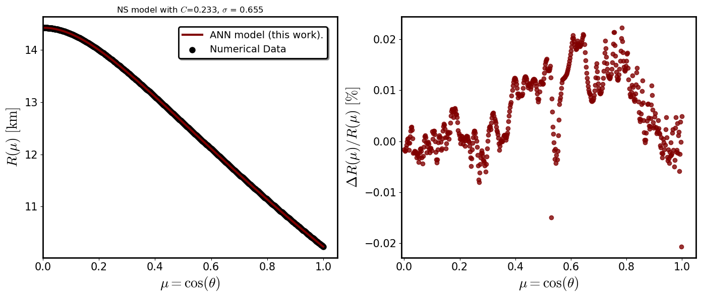
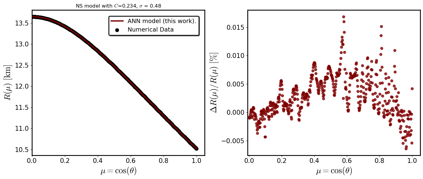
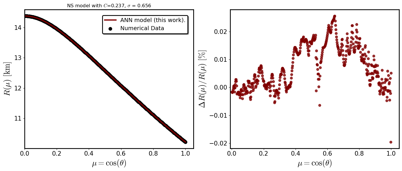
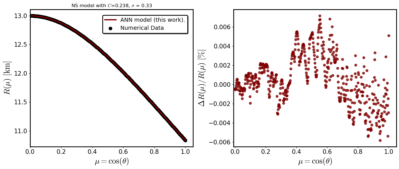
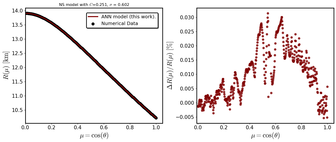
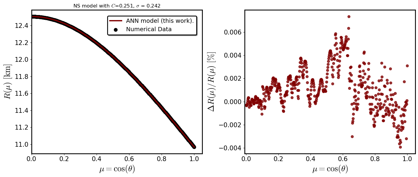
Visualization of the all the surface curves in the selected set (Train/Test) dataset for the specific EOS loaded

def calculate_model_estimation(C, sigma, R_pole, R_eq):
    num = 50
    mu = np.linspace(0, 1, num=num, dtype=np.float32)
    C_np = np.array([C for _ in range(0, num)], dtype=np.float32)
    sigma_np = np.array([sigma for _ in range(0, num)], dtype=np.float32)
    e_np = np.array([np.sqrt(1 - np.square(R_pole / R_eq)) for _ in range(0, num)], dtype=np.float32)
    x = torch.tensor(np.array([mu, C_np, sigma_np, e_np])).T.to(device) # Convert the argument list to array for optimization 
    model_estimation = regressor(x) * (R_eq - R_pole) + R_pole
    model_estimation = model_estimation.cpu().detach().numpy()
    
    ##########################################################################
    #Convert the estimation list to 1-d array with dtype float 32 in order 
    #to have the same dimenensions and dtype with mu = cos(theta)
    model_estimation = model_estimation.ravel().astype(np.float32)
    ##########################################################################
    
    return mu, model_estimation

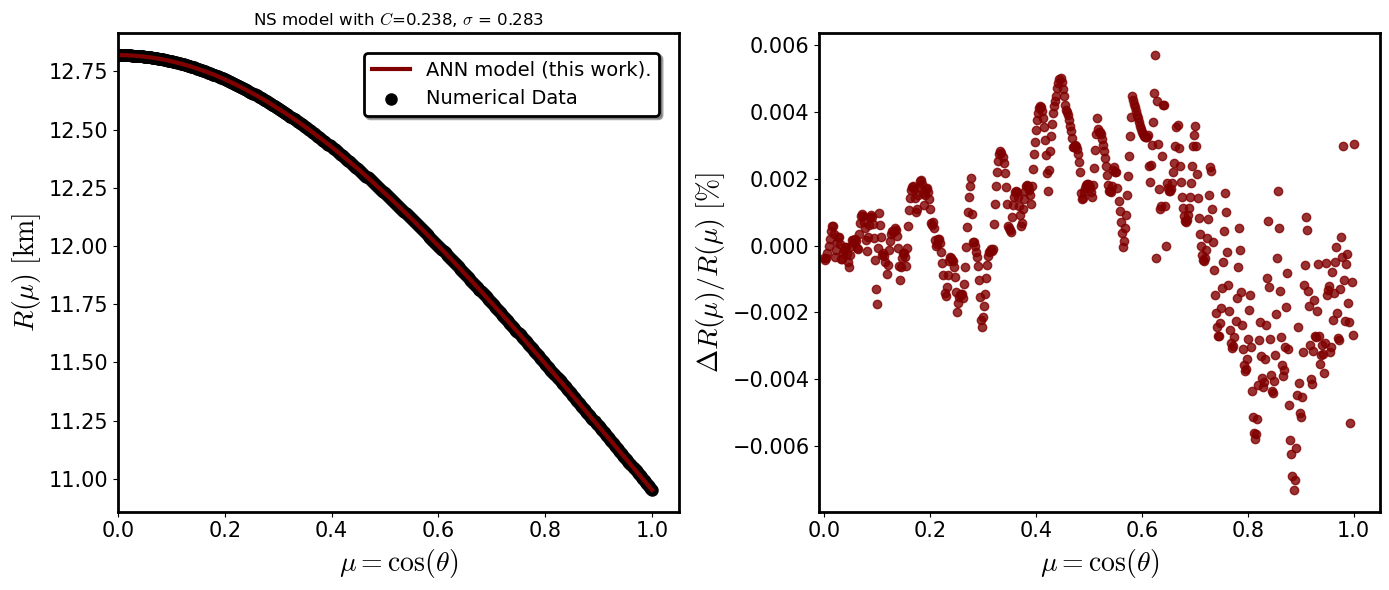
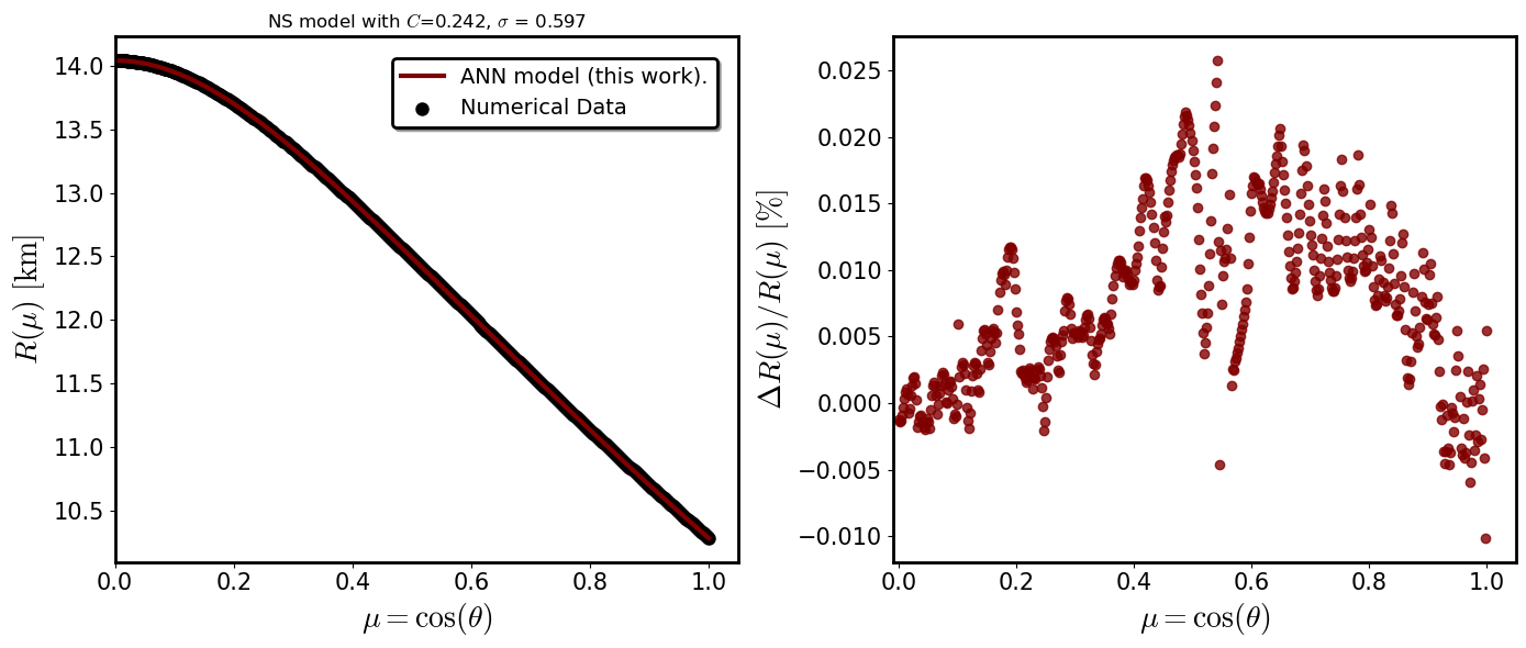
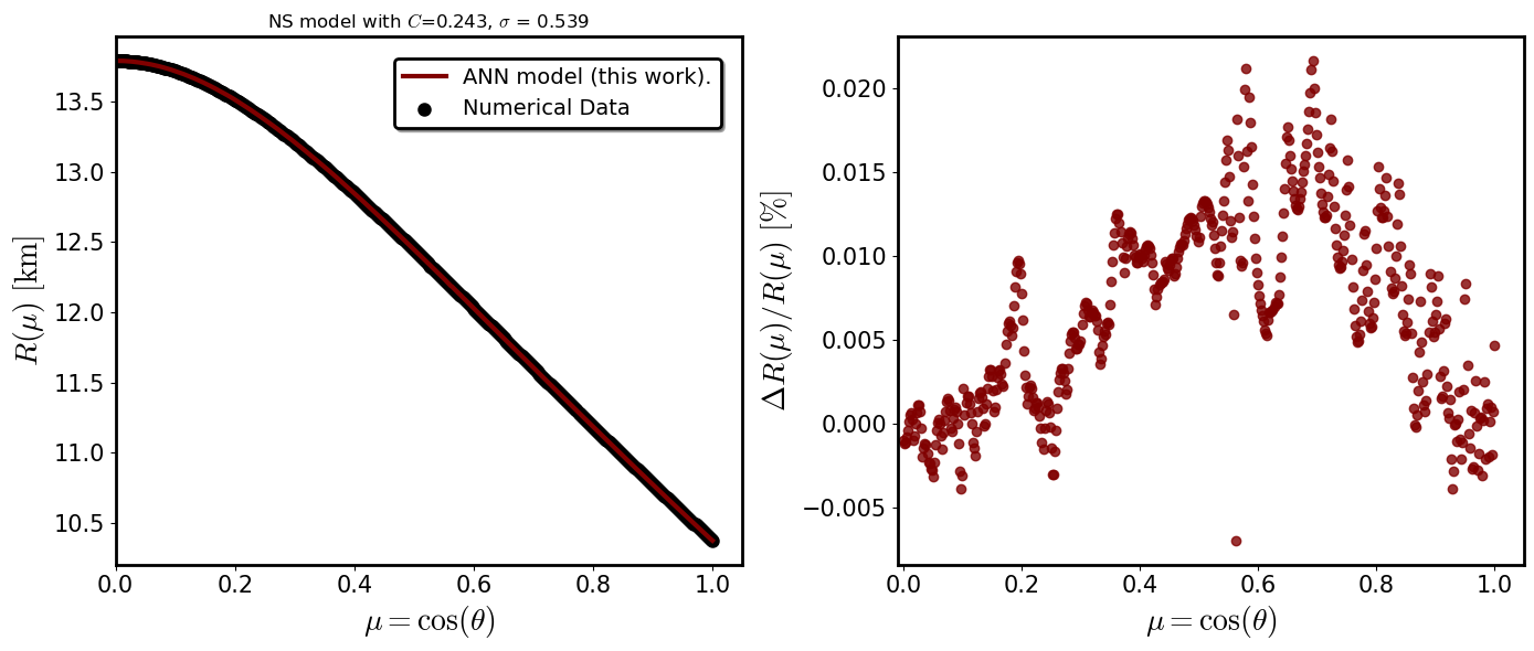
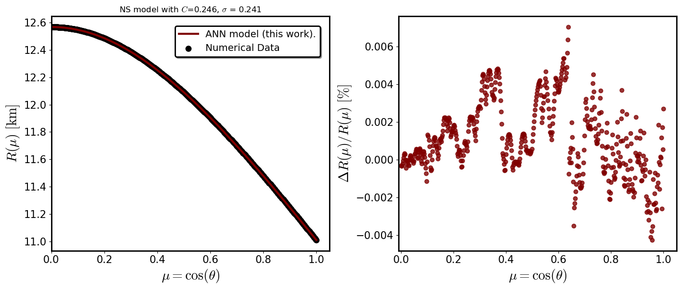
# Select Training or test set
is_train = False # True or False

select_set = lambda is_train, df_train, df_test: df_train if is_train else df_test
select_features = lambda is_train, np_features_tr, np_features_ts: np_features_tr if is_train else np_features_ts
select_targets = lambda is_train, np_targets_tr, np_targets_ts: np_targets_tr if is_train else np_targets_ts
    
# Select Set (Train/Test)
df_set = select_set(is_train, df_train, df_test)
features = select_features(is_train, np_features_tr, np_features_ts)
targets = select_targets(is_train, np_targets_tr, np_targets_ts)
    
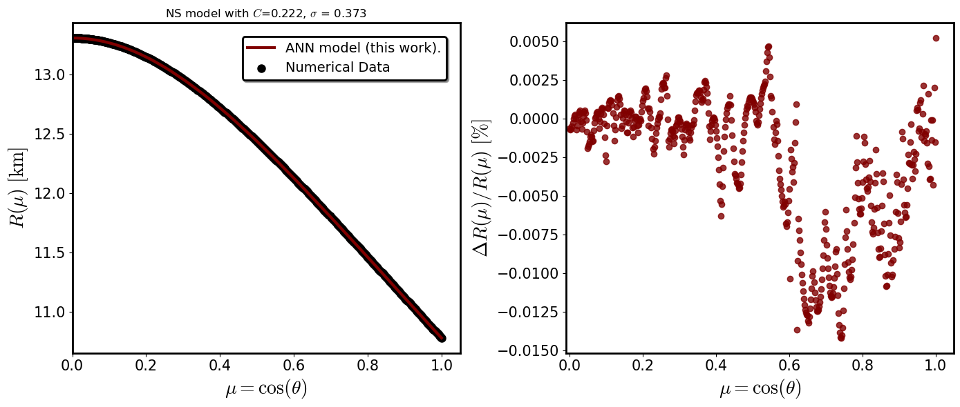
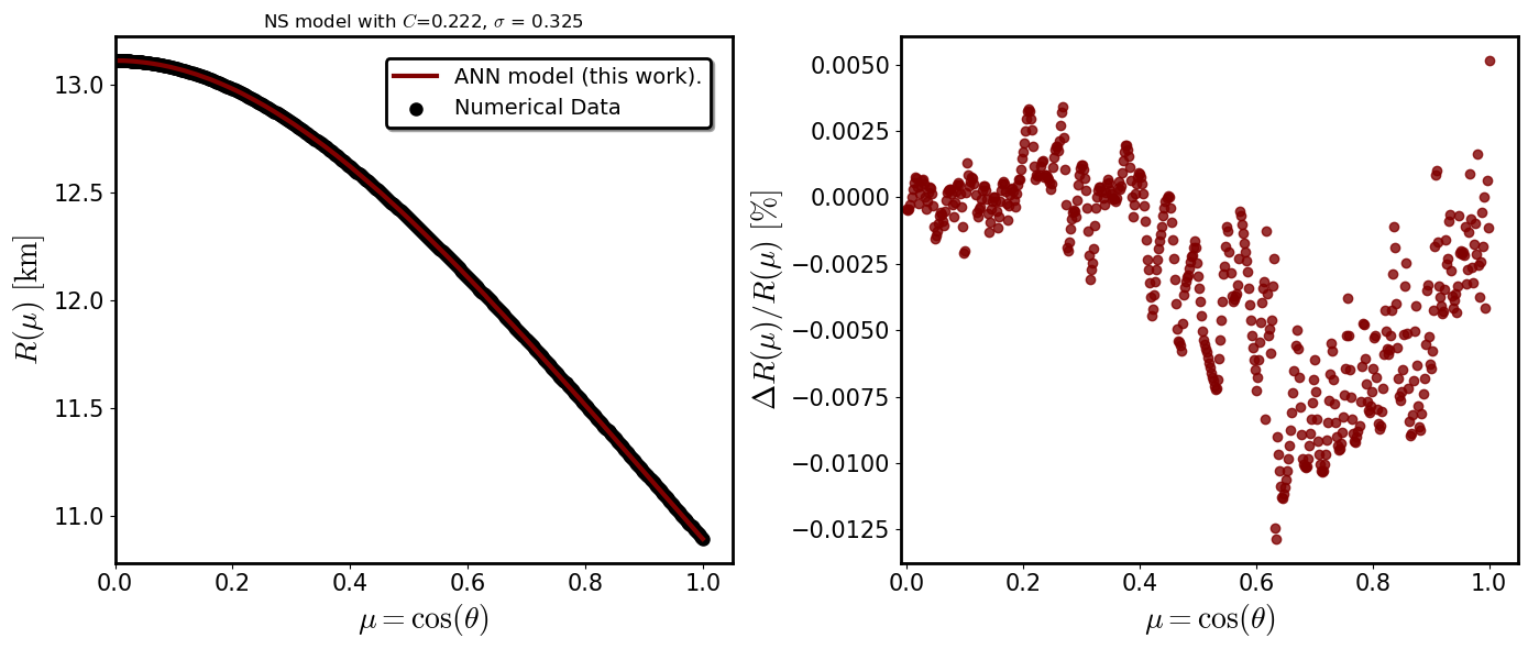
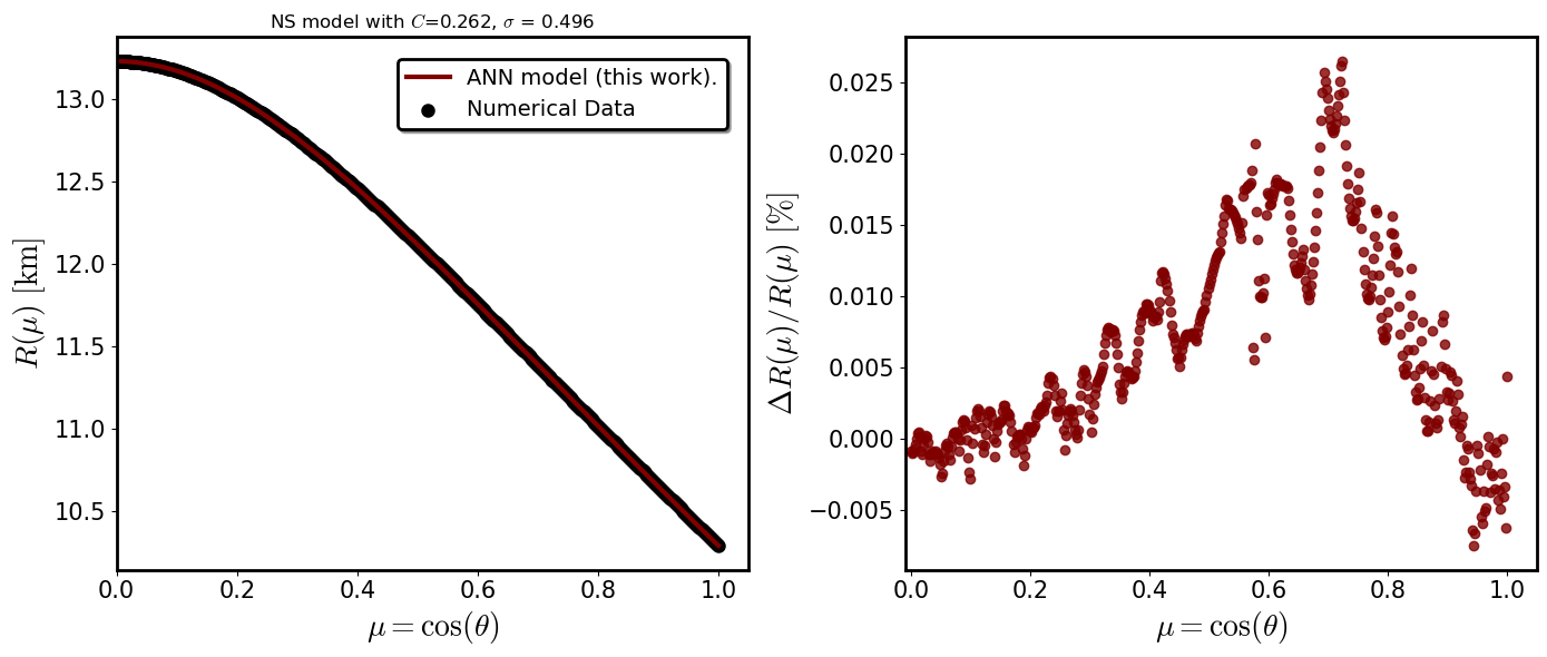
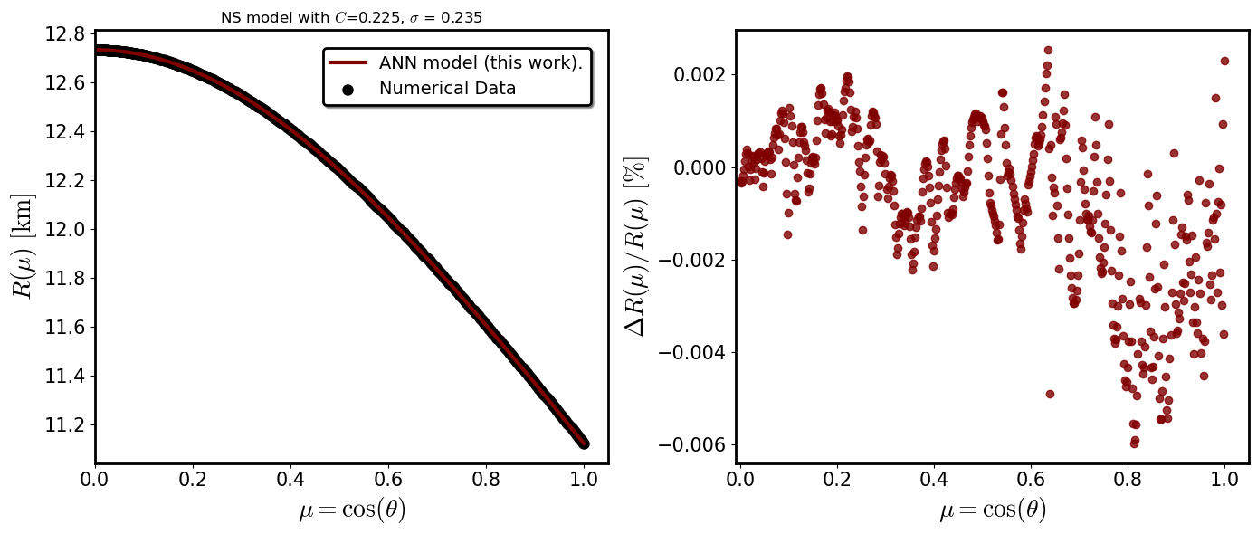
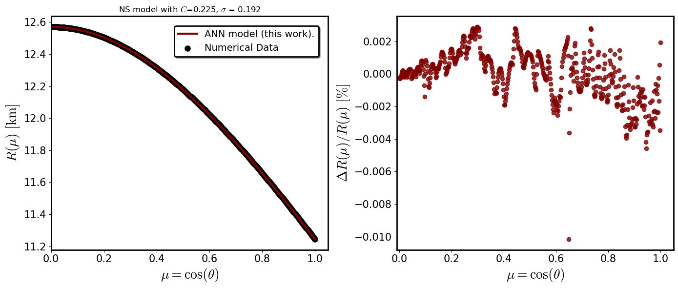
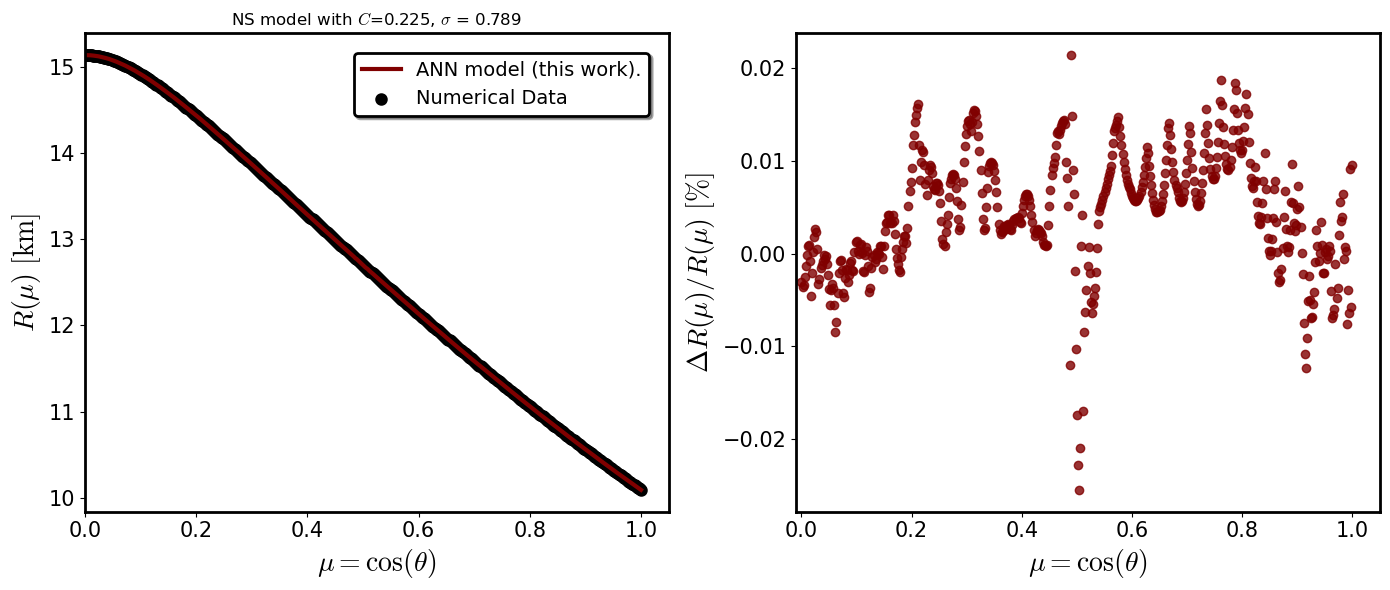
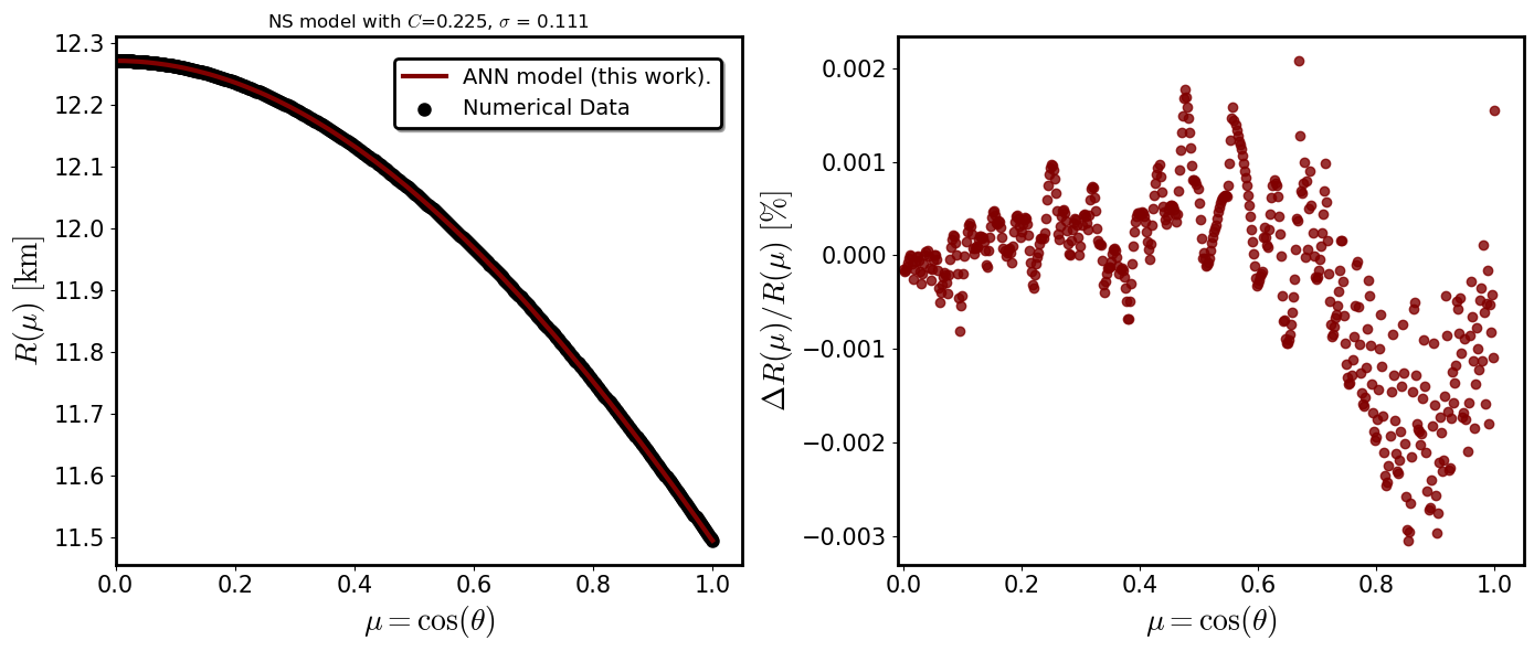
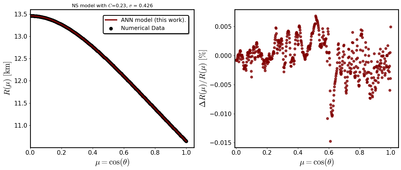
for star_index in range(0, 150):
    # Do not change
    low = star_index * N_MU
    high = (star_index + 1) * N_MU
    mu = df_set['cos(theta)'].iloc[low:high]
    
    
    # Transformed estimations and targets to kilometers 
    estimation = regressor.predict(features[low:high])
    ##########################################################################
    #Convert the estimation list to 1-d array with dtype float 64 in order 
    #to have the same dimenensions and dtype with mu = cos(theta)
    estimation = estimation.ravel().astype(np.float64) 
    ##########################################################################
    maxmin_diff = df_set['Req_num'].iloc[low] - df_set['Rpole_num'].iloc[low]
    min_ = df_set['Rpole_num'].iloc[low]
    
    # Using the universal relations provided:
    #maxmin_diff = df_set['Req_num'].iloc[low] -  R_pole(df_set['Req_num'].iloc[low], C, sigma)
    #min_ = R_pole(df_set['Req_num'].iloc[low], C, sigma)
   
    
    # Static case
    if np.all(df_set[spin].iloc[low:high] == 0):
        model_estimation = estimation * df_set['Req_num'].iloc[low]
        real_targets = targets[low:high] * df_set['Req_num'].iloc[low]
    # Rotational case
    else:
        model_estimation = estimation * (maxmin_diff) + min_ 
        real_targets = targets[low:high] * (maxmin_diff) + min_
    real_targets = real_targets.ravel()
    
    ANN_fract_diff = 100*(model_estimation - real_targets)/real_targets
   
    ############# Req, C and sigma for each star ######################################
    C = df_set['C'].iloc[low]
    sigma = df_set['sigma'].iloc[low]
    R_eq = df_set['Req_num'].iloc[low]
    
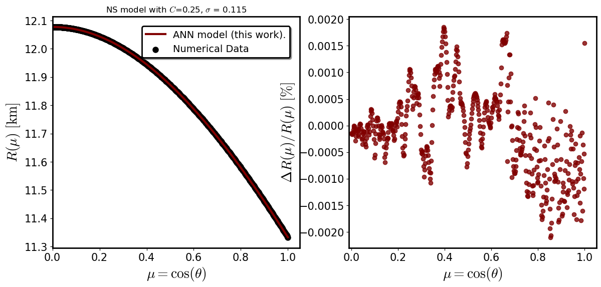
    # Create two subplots side by side
    fig, axs = plt.subplots(1, 2, figsize=(14, 6))
        
    # Plot the first graph in the left subplot
    axs[0].plot(mu, model_estimation, lw=3, c='maroon', label='ANN model (this work).')
    axs[0].scatter(mu, real_targets, lw=3, c='black', label='Numerical Data')
    
    axs[0].set_xlabel(r'$\mu = \cos(\theta)$', fontsize=20)
    axs[0].set_ylabel(r'$R(\mu) \ [\mathrm{km}]$', fontsize=20)
    axs[0].set_title(f'NS model with $C$={round(C,3)}, $\sigma$ = {round(sigma,3)}')
    axs[0].legend(loc='best', prop={'size': 15}, shadow=True, fontsize='large')
    axs[0].tick_params(axis='both', which='both', labelsize=15)

    axs[0].set_xlim(0,None)

    for axis in ['top','bottom','left','right']:
        axs[0].spines[axis].set_linewidth(2.0)

    leg = axs[0].legend(loc="best",ncol=1, borderaxespad=1, prop={'size': 14}, shadow=True, fontsize="large") 
    leg.get_frame().set_linewidth(2.0)
    leg.get_frame().set_edgecolor('black')
    

    axs[1].scatter(mu, ANN_fract_diff , lw=1, alpha = 0.8, c='maroon')
    axs[1].set_xlabel(r'$ \mu = \cos(\theta)$', fontsize=20)
    axs[1].set_ylabel(r'$\Delta R(\mu)/ R(\mu) \ [\%]$', fontsize=20)
    axs[1].tick_params(axis='both', which='both', labelsize=15)


    for axis in ['top','bottom','left','right']:
        axs[1].spines[axis].set_linewidth(2.0)

    axs[1].set_xlim(-0.01,None)

    
    plt.tight_layout()
    plt.show()

 

---------------------------------------------------------------------------
KeyboardInterrupt                         Traceback (most recent call last)
Cell In[28], line 87
     82     axs[1].spines[axis].set_linewidth(2.0)
     84 axs[1].set_xlim(-0.01,None)
---> 87 plt.tight_layout()
     88 plt.show()

File ~/anaconda3/lib/python3.11/site-packages/matplotlib/pyplot.py:2587, in tight_layout(pad, h_pad, w_pad, rect)
   2579 @_copy_docstring_and_deprecators(Figure.tight_layout)
   2580 def tight_layout(
   2581     *,
   (...)
   2585     rect: tuple[float, float, float, float] | None = None,
   2586 ) -> None:
-> 2587     gcf().tight_layout(pad=pad, h_pad=h_pad, w_pad=w_pad, rect=rect)

File ~/anaconda3/lib/python3.11/site-packages/matplotlib/figure.py:3540, in Figure.tight_layout(self, pad, h_pad, w_pad, rect)
   3538 previous_engine = self.get_layout_engine()
   3539 self.set_layout_engine(engine)
-> 3540 engine.execute(self)
   3541 if previous_engine is not None and not isinstance(
   3542     previous_engine, (TightLayoutEngine, PlaceHolderLayoutEngine)
   3543 ):
   3544     _api.warn_external('The figure layout has changed to tight')

File ~/anaconda3/lib/python3.11/site-packages/matplotlib/layout_engine.py:183, in TightLayoutEngine.execute(self, fig)
    181 renderer = fig._get_renderer()
    182 with getattr(renderer, "_draw_disabled", nullcontext)():
--> 183     kwargs = get_tight_layout_figure(
    184         fig, fig.axes, get_subplotspec_list(fig.axes), renderer,
    185         pad=info['pad'], h_pad=info['h_pad'], w_pad=info['w_pad'],
    186         rect=info['rect'])
    187 if kwargs:
    188     fig.subplots_adjust(**kwargs)

File ~/anaconda3/lib/python3.11/site-packages/matplotlib/_tight_layout.py:266, in get_tight_layout_figure(fig, axes_list, subplotspec_list, renderer, pad, h_pad, w_pad, rect)
    261         return {}
    262     span_pairs.append((
    263         slice(ss.rowspan.start * div_row, ss.rowspan.stop * div_row),
    264         slice(ss.colspan.start * div_col, ss.colspan.stop * div_col)))
--> 266 kwargs = _auto_adjust_subplotpars(fig, renderer,
    267                                   shape=(max_nrows, max_ncols),
    268                                   span_pairs=span_pairs,
    269                                   subplot_list=subplot_list,
    270                                   ax_bbox_list=ax_bbox_list,
    271                                   pad=pad, h_pad=h_pad, w_pad=w_pad)
    273 # kwargs can be none if tight_layout fails...
    274 if rect is not None and kwargs is not None:
    275     # if rect is given, the whole subplots area (including
    276     # labels) will fit into the rect instead of the
   (...)
    280     # auto_adjust_subplotpars twice, where the second run
    281     # with adjusted rect parameters.

File ~/anaconda3/lib/python3.11/site-packages/matplotlib/_tight_layout.py:82, in _auto_adjust_subplotpars(fig, renderer, shape, span_pairs, subplot_list, ax_bbox_list, pad, h_pad, w_pad, rect)
     80 for ax in subplots:
     81     if ax.get_visible():
---> 82         bb += [martist._get_tightbbox_for_layout_only(ax, renderer)]
     84 tight_bbox_raw = Bbox.union(bb)
     85 tight_bbox = fig.transFigure.inverted().transform_bbox(tight_bbox_raw)

File ~/anaconda3/lib/python3.11/site-packages/matplotlib/artist.py:1411, in _get_tightbbox_for_layout_only(obj, *args, **kwargs)
   1405 """
   1406 Matplotlib's `.Axes.get_tightbbox` and `.Axis.get_tightbbox` support a
   1407 *for_layout_only* kwarg; this helper tries to use the kwarg but skips it
   1408 when encountering third-party subclasses that do not support it.
   1409 """
   1410 try:
-> 1411     return obj.get_tightbbox(*args, **{**kwargs, "for_layout_only": True})
   1412 except TypeError:
   1413     return obj.get_tightbbox(*args, **kwargs)

File ~/anaconda3/lib/python3.11/site-packages/matplotlib/_api/deprecation.py:454, in make_keyword_only.<locals>.wrapper(*args, **kwargs)
    448 if len(args) > name_idx:
    449     warn_deprecated(
    450         since, message="Passing the %(name)s %(obj_type)s "
    451         "positionally is deprecated since Matplotlib %(since)s; the "
    452         "parameter will become keyword-only %(removal)s.",
    453         name=name, obj_type=f"parameter of {func.__name__}()")
--> 454 return func(*args, **kwargs)

File ~/anaconda3/lib/python3.11/site-packages/matplotlib/axes/_base.py:4395, in _AxesBase.get_tightbbox(self, renderer, call_axes_locator, bbox_extra_artists, for_layout_only)
   4393 for axis in self._axis_map.values():
   4394     if self.axison and axis.get_visible():
-> 4395         ba = martist._get_tightbbox_for_layout_only(axis, renderer)
   4396         if ba:
   4397             bb.append(ba)

File ~/anaconda3/lib/python3.11/site-packages/matplotlib/artist.py:1411, in _get_tightbbox_for_layout_only(obj, *args, **kwargs)
   1405 """
   1406 Matplotlib's `.Axes.get_tightbbox` and `.Axis.get_tightbbox` support a
   1407 *for_layout_only* kwarg; this helper tries to use the kwarg but skips it
   1408 when encountering third-party subclasses that do not support it.
   1409 """
   1410 try:
-> 1411     return obj.get_tightbbox(*args, **{**kwargs, "for_layout_only": True})
   1412 except TypeError:
   1413     return obj.get_tightbbox(*args, **kwargs)

File ~/anaconda3/lib/python3.11/site-packages/matplotlib/axis.py:1334, in Axis.get_tightbbox(self, renderer, for_layout_only)
   1332 if renderer is None:
   1333     renderer = self.figure._get_renderer()
-> 1334 ticks_to_draw = self._update_ticks()
   1336 self._update_label_position(renderer)
   1338 # go back to just this axis's tick labels

File ~/anaconda3/lib/python3.11/site-packages/matplotlib/axis.py:1277, in Axis._update_ticks(self)
   1275 major_locs = self.get_majorticklocs()
   1276 major_labels = self.major.formatter.format_ticks(major_locs)
-> 1277 major_ticks = self.get_major_ticks(len(major_locs))
   1278 for tick, loc, label in zip(major_ticks, major_locs, major_labels):
   1279     tick.update_position(loc)

File ~/anaconda3/lib/python3.11/site-packages/matplotlib/axis.py:1628, in Axis.get_major_ticks(self, numticks)
   1626     tick = self._get_tick(major=True)
   1627     self.majorTicks.append(tick)
-> 1628     self._copy_tick_props(self.majorTicks[0], tick)
   1630 return self.majorTicks[:numticks]

File ~/anaconda3/lib/python3.11/site-packages/matplotlib/axis.py:1580, in Axis._copy_tick_props(self, src, dest)
   1578 if src is None or dest is None:
   1579     return
-> 1580 dest.label1.update_from(src.label1)
   1581 dest.label2.update_from(src.label2)
   1582 dest.tick1line.update_from(src.tick1line)

File ~/anaconda3/lib/python3.11/site-packages/matplotlib/text.py:356, in Text.update_from(self, other)
    354 self._linespacing = other._linespacing
    355 self._antialiased = other._antialiased
--> 356 self.stale = True

File ~/anaconda3/lib/python3.11/site-packages/matplotlib/artist.py:317, in Artist.stale(self, val)
    311     """
    312     Whether the artist is 'stale' and needs to be re-drawn for the output
    313     to match the internal state of the artist.
    314     """
    315     return self._stale
--> 317 @stale.setter
    318 def stale(self, val):
    319     self._stale = val
    321     # if the artist is animated it does not take normal part in the
    322     # draw stack and is not expected to be drawn as part of the normal
    323     # draw loop (when not saving) so do not propagate this change

KeyboardInterrupt: